Page 152 - Separation process engineering

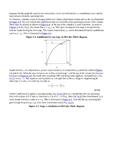
diagram. On this graph the equilibrium relationship can be solved from the y-x equilibrium curve and the
mass balances from the operating lines.

To illustrate, consider a typical design problem for a binary distillation column such as the one illustrated
in Figure 3-8. We will assume that equilibrium data are available at the operating pressure of the column.
These data are plotted as shown in Figure 4-4. At the top of the column is a total condenser. As noted in
Chapter 3 in Eq. (3-7), this means that y = x = x . The vapor leaving the first stage is in equilibrium
1 D 0
with the liquid leaving the first stage. This liquid composition, x , can be determined from the equilibrium
1
curve at y = y . This is illustrated in Figure 4-4.
1
Figure 4-4. Equilibrium for top stage on McCabe-Thiele diagram

Liquid stream L of composition x passes vapor stream V of composition y inside the column (Figures
2
1
1
2
3-8 and 4-1A). When the mass balances are written around stage 1 and the top of the column (see balance
envelope in Figure 4-1A), the result after assuming CMO and doing some algebraic manipulations is Eq.
(4-12) with j = 1. This equation can be plotted as a straight line on the y-x diagram. Suppressing the
subscripts j+1 and j, we write Eq. (4-12b) as

(4-21)

which is understood to apply to passing streams. Eq. (4-21) plots as a straight line (the top operating
line) with a slope of L/V and a y intercept (x = 0) of (1 − L/V)x . Once Eq. (4-12) has been plotted, y is
2
D
easily found from the y value at x = x . This is illustrated in Figure 4-5. Note that the top operating line
1
goes through the point (y , x ) since these coordinates satisfy Eq. (4-21).
D
1
Figure 4-5. Stage 1 calculation on McCabe-Thiele diagram