Page 151 -

148 G. Polhill

3
not be justified. There may be a way to assess the question of the ‘power’ a system
of interacting agents has to realize different ‘shapes’ from input to output (however,
that is understood in an ABM context) quantitatively. In the early 1970s, Vapnik
and Chervonenkis (1971) published a paper that provided a lower bound on the
probability that the difference between the actual predictive power of a classifier
system and that estimated from calibration is more than a small amount, based
on the amount of data it is given and something called the ‘Vapnik-Chervonenkis
dimension’ of the classifier. The inequality is written thus (Vapnik and Chervonenkis
1971, p. 269):

2
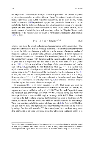
P .jg hj >"/ 4m.2n/e " n=8 (8.1)
where g and h are the actual and estimated generalization ability, respectively (the
proportion of instances that are correctly classified), " is the small amount we want
to bound the difference between g and h to, n is the amount of data (as number of
instances) and m(x) is a function that tells you the number of different realizations
x
the classifier can make on x datapoints. The function m() is equal to 2 until x D d VC ,
the Vapnik-Chervonenkis (VC) dimension of the classifier, after which it continues
x
to grow but at a polynomial rate less than 2 and no more than x d VC C 1 (Hertz
et al. 1991, p. 154). A rough idea of the shape of the growth function m() can be
seen in Fig. 8.1, particularly the red (top) curve when d VC D 4. In a log-log plot,
m() is convex until a critical point at which it becomes linear; as stated above, this
critical point is the VC dimension of the function d VC , but the red curve in Fig. 8.1
is 4 m(2n), so in fact the critical point on the red curve should be at n D 0.5d VC .
x
However, since x d VC C 1>2 for lower values of x, the polynomial upper bound
on m() isn’t informative; the critical point in Fig. 8.1 at which m() becomes linear is
therefore higher than would otherwise be expected.
To understand (8.1) a bit better, imagine " D 0.01. That means you want the
difference between the actual and estimated abilities to be less than 0.01 ideally. So,
suppose you have a validation ability (h) of 0.95 (5% of the model’s predictions on
the validation data are wrong); then with " D 0.01, you are saying you want your
future predictions to have an ability (g) in the range [0.94, 0.96]. How certain do
you want to be that you have achieved that? Suppose you want to be at least 99.9%
certain, so one in a thousand predictions will have an ability outside the above range.
Then you want the probability on the left-hand side of (8.1), P, to be 0.001. How
can you achieve this? The right-hand side says that the probability can be reduced
by using a function with a smaller VC dimension (so m(2n) is smaller), using more
data (increasing n) or being less fussy about how close your validation ability is to

3
Part of this is the confusion between ‘free parameters’, which can be adjusted to make the results
fit data, and parameters with values that are, at least in theory, empirically observable, even if
currently unknown. Agent-based models have a lot of the latter but relatively few of the former.