Page 212 -

10 Understanding Simulation Results 209

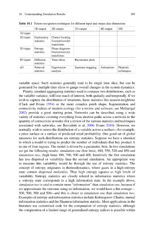
Table 10.1 Pattern recognition techniques for different input and output data dimensions
1D output 2D output 3D output 4D output ND
1D input
2D input Exploratory Cluster locating
statistics Fourier/wavelet
transforms
3D input Entropy Phase diagrams
statistics Fourier/wavelet
transforms
4D input Diffusion Time slices Recurrence plots
statistics
nD Network Eigenvector Sammon mapping Animations Heuristic
statistics analysis techniques

variable space. Such statistics generally tend to be single time slice, but can be
generated for multiple time slices to gauge overall changes in the system dynamics.
Plainly, standard aggregating statistics used to compare two distributions, such as
the variable variance, will lose much of interest, both spatially and temporally. If we
wish to capture the distribution of invariants, basic statistics like nearest-neighbour
(Clark and Evans 1954) or the more complex patch shape, fragmentation and
connectivity indices of modern ecology (for a review and software, see McGarigal
2002) provide a good starting point. Networks can be described using a wide
variety of statistics covering everything from shortest paths across a network to the
quantity of connections at nodes (for a review of the various statistics and techniques
associated with networks, see Boccaletti et al. 2006; Evans 2010). However, we
normally wish to assess the distribution of a variable across a surface—for example,
a price surface or a surface of predicted retail profitability. One good set of global
measures for such distributions are entropy statistics. Suppose we have a situation
in which a model is trying to predict the number of individuals that buy product A
in one of four regions. The model is driven by a parameter, beta. In two simulations
we get the following results: simulation one (low beta), 480, 550, 520 and 450 and
simulation two, (high beta) 300, 700, 500 and 400. Intuitively the first simulation
has less dispersal or variability than the second simulation. An appropriate way
to measure this variability would be through the use of entropy statistics. The
concept of entropy originates in thermodynamics, where gases in a high-entropy
state contain dispersed molecules. Thus high entropy equates to high levels of
variability. Entropy statistics are closely related to information statistics where
a -entropy state corresponds to a high information state. In the example above,
simulation two is said to contain more “information” than simulation one, because if
we approximate the outcome using no information, we would have a flat average—
500, 500, 500 and 500—and this is closer to simulation one than simulation two.
Examples of entropy and information statistics include Kolmogorov-Chaitin, mutual
information statistics and the Shannon information statistic. Most applications in the
literature use customised code for the computation of entropy statistics, although
the computation of a limited range of generalised entropy indices is possible within