Page 152 -

135

as measured in terms of then the flow away from the wall is t = 1, with only
exponentially small corrections. The boundary layer remains thin along
the full length of the pipe, but note that lines of constant temperature, emanating
from the neighbourhood of the wall, are the lines i.e.
Thus, defining the boundary-layer thickness in terms of a particular temperature, this
thickness increases as x increases, although it remains However,
if the pipe is so long that then the exponential term in (3.59) becomes
O(1), and the temperature now has an O(1) correction. In other words, the O(1)
temperature at the pipe wall has caused heat to be conducted through the fluid to
affect the whole pipe flow, Indeed, we see that the scaling in our
original equation, (3.53), balances dominant terms from both sides of the equation for
there is no longer a boundary layer at the wall; this is shown schematically
in figure 5.

The two examples presented above have shown how the notion of a boundary
layer, as developed for ordinary differential equations, is relevant to partial differen-
tial equations—and essentially without any adjustment to the method; some similar
examples can be found in exercises Q3.12–3.14. We have now seen the two basic
types of problem (breakdown and rescale; select a scaling relevant to a layer), although
the equations that we have introduced as the vehicles for these demonstrations—quite
deliberately—have been relatively uncomplicated. We conclude this section with an
example that, ultimately, possesses a simple perturbation structure (as in §3.2), but
which involves a set of four, coupled, nonlinear partial differential equations. As be-
fore, the purpose of the example is to exhibit the power (and inherent simplicity) of
the singular perturbation approach.

E3.5 Unsteady, one-dimensional flow of a viscous, compressible gas
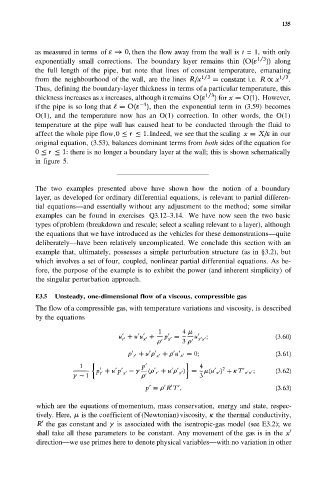
The flow of a compressible gas, with temperature variations and viscosity, is described
by the equations

which are the equations of momentum, mass conservation, energy and state, respec-
tively. Here, is the coefficient of (Newtonian) viscosity, the thermal conductivity,
the gas constant and is associated with the isentropic-gas model (see E3.2); we
shall take all these parameters to be constant. Any movement of the gas is in the
direction—we use primes here to denote physical variables—with no variation in other