Page 148 -

131

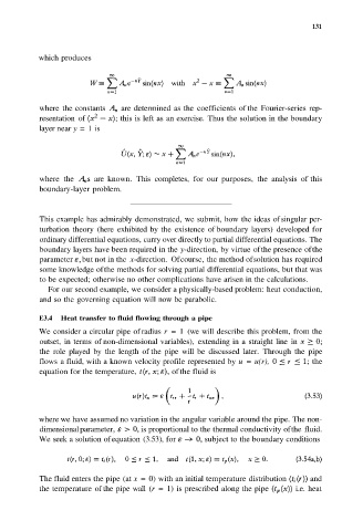
which produces

where the constants are determined as the coefficients of the Fourier-series rep-
resentation of this is left as an exercise. Thus the solution in the boundary
layer near y = 1 is

where the are known. This completes, for our purposes, the analysis of this
boundary-layer problem.

This example has admirably demonstrated, we submit, how the ideas of singular per-
turbation theory (here exhibited by the existence of boundary layers) developed for
ordinary differential equations, carry over directly to partial differential equations. The
boundary layers have been required in the y-direction, by virtue of the presence of the
parameter but not in the x-direction. Of course, the method of solution has required
some knowledge of the methods for solving partial differential equations, but that was
to be expected; otherwise no other complications have arisen in the calculations.
For our second example, we consider a physically-based problem: heat conduction,
and so the governing equation will now be parabolic.

E3.4 Heat transfer to fluid flowing through a pipe
We consider a circular pipe of radius r = 1 (we will describe this problem, from the
outset, in terms of non-dimensional variables), extending in a straight line in
the role played by the length of the pipe will be discussed later. Through the pipe
flows a fluid, with a known velocity profile represented by u = u(r), the
equation for the temperature, of the fluid is

where we have assumed no variation in the angular variable around the pipe. The non-
dimensional parameter, is proportional to the thermal conductivity of the fluid.
We seek a solution of equation (3.53), for subject to the boundary conditions

The fluid enters the pipe (at x = 0) with an initial temperature distribution and
the temperature of the pipe wall (r = 1) is prescribed along the pipe i.e. heat