Page 176 -

159

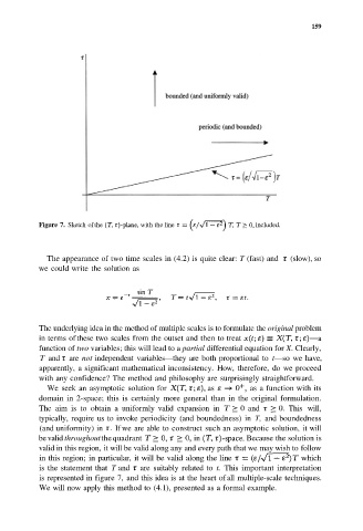
Figure 7. Sketch of the with the line included.

The appearance of two time scales in (4.2) is quite clear: T (fast) and (slow), so
we could write the solution as

The underlying idea in the method of multiple scales is to formulate the original problem
in terms of these two scales from the outset and then to treat
function of two variables; this will lead to a partial differential equation for X. Clearly,
T and are not independent variables—they are both proportional to t—so we have,
apparently, a significant mathematical inconsistency. How, therefore, do we proceed
with any confidence? The method and philosophy are surprisingly straightforward.
We seek an asymptotic solution for as as a function with its
domain in 2-space; this is certainly more general than in the original formulation.
The aim is to obtain a uniformly valid expansion in and This will,
typically, require us to invoke periodicity (and boundedness) in T, and boundedness
(and uniformity) in If we are able to construct such an asymptotic solution, it will
be valid throughout the quadrant in Because the solution is
valid in this region, it will be valid along any and every path that we may wish to follow
in this region; in particular, it will be valid along the line which
is the statement that T and are suitably related to t. This important interpretation
is represented in figure 7, and this idea is at the heart of all multiple-scale techniques.
We will now apply this method to (4.1), presented as a formal example.