Page 92 -

75

for but that solutions obtained from these expansions may diverge as
we may have x = 0 in the domain, but

The examples that we have presented thus far (and others can be found in Q2.11-2.15),
and particularly those that involve a rescaling after a breakdown, possess an important
but rather less obvious property. This relates to the existence of general scalings of the
differential equation, and the resulting ‘balance’ of (dominant) terms in the equation;
this leads us to the introduction of an additional fundamental tool. This idea will now
be explored in some detail, and use made of it in some further examples.

2.5 SCALING OF DIFFERENTIAL EQUATIONS
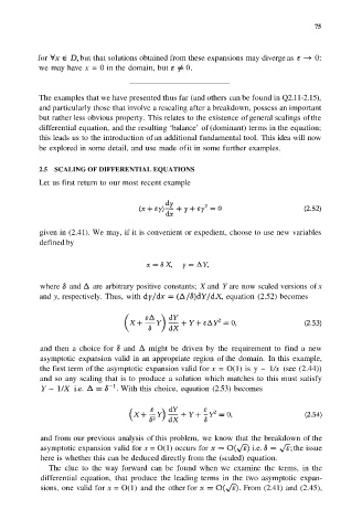
Let us first return to our most recent example

given in (2.41). We may, if it is convenient or expedient, choose to use new variables
defined by

where and are arbitrary positive constants; X and Y are now scaled versions of x
and y, respectively. Thus, with equation (2.52) becomes

and then a choice for and might be driven by the requirement to find a new
asymptotic expansion valid in an appropriate region of the domain. In this example,
the first term of the asymptotic expansion valid for x = O(1) is y ~ 1/x (see (2.44))
and so any scaling that is to produce a solution which matches to this must satisfy
Y ~ 1/X i.e. With this choice, equation (2.53) becomes

and from our previous analysis of this problem, we know that the breakdown of the
asymptotic expansion valid for x = O(1) occurs for i.e. the issue
here is whether this can be deduced directly from the (scaled) equation.
The clue to the way forward can be found when we examine the terms, in the
differential equation, that produce the leading terms in the two asymptotic expan-
sions, one valid for x = O(1) and the other for From (2.41) and (2.45),