Page 96 -

79

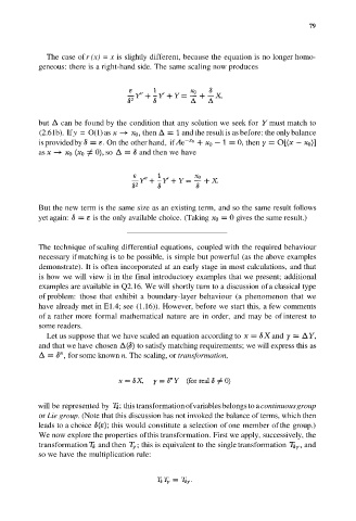
The case of r (x) = x is slightly different, because the equation is no longer homo-
geneous: there is a right-hand side. The same scaling now produces

but can be found by the condition that any solution we seek for Y must match to
(2.61b). If y = O(1) as then and the result is as before: the only balance
is provided by On the other hand, if then
as so and then we have

But the new term is the same size as an existing term, and so the same result follows
yet again: is the only available choice. (Taking gives the same result.)

The technique of scaling differential equations, coupled with the required behaviour
necessary if matching is to be possible, is simple but powerful (as the above examples
demonstrate). It is often incorporated at an early stage in most calculations, and that
is how we will view it in the final introductory examples that we present; additional
examples are available in Q2.16. We will shortly turn to a discussion of a classical type
of problem: those that exhibit a boundary-layer behaviour (a phenomenon that we
have already met in E1.4; see (1.16)). However, before we start this, a few comments
of a rather more formal mathematical nature are in order, and may be of interest to
some readers.
Let us suppose that we have scaled an equation according to and
and that we have chosen to satisfy matching requirements; we will express this as
for some known n. The scaling, or transformation,

will be represented by this transformation of variables belongs to a continuous group
or Lie group. (Note that this discussion has not invoked the balance of terms, which then
leads to a choice this would constitute a selection of one member of the group.)
We now explore the properties of this transformation. First we apply, successively, the
transformation and then this is equivalent to the single transformation and
so we have the multiplication rule: