Page 185 - Six Sigma Demystified

Chapter 7 i m p r o v e S tag e 165

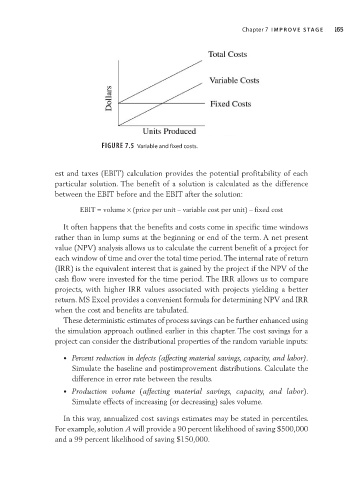
FiguRe 7.5 Variable and fixed costs.

est and taxes (EBIT) calculation provides the potential profitability of each
particular solution. The benefit of a solution is calculated as the difference
between the EBIT before and the EBIT after the solution:

EBIT = volume × (price per unit – variable cost per unit) – fixed cost

It often happens that the benefits and costs come in specific time windows
rather than in lump sums at the beginning or end of the term. A net present
value (NPV) analysis allows us to calculate the current benefit of a project for
each window of time and over the total time period. The internal rate of return
(IRR) is the equivalent interest that is gained by the project if the NPV of the
cash flow were invested for the time period. The IRR allows us to compare
projects, with higher IRR values associated with projects yielding a better
return. MS Excel provides a convenient formula for determining NPV and IRR
when the cost and benefits are tabulated.

These deterministic estimates of process savings can be further enhanced using
the simulation approach outlined earlier in this chapter. The cost savings for a
project can consider the distributional properties of the random variable inputs:

• Percent reduction in defects (affecting material savings, capacity, and labor).
Simulate the baseline and postimprovement distributions. Calculate the
difference in error rate between the results.

• Production volume (affecting material savings, capacity, and labor).
Simulate effects of increasing (or decreasing) sales volume.

In this way, annualized cost savings estimates may be stated in percentiles.
For example, solution A will provide a 90 percent likelihood of saving $500,000
and a 99 percent likelihood of saving $150,000.