Page 380 - Six Sigma Demystified

360 Six SigMa DemystifieD

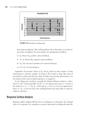
Figure F.39 Example of a residuals plot.

tion (autocorrelation). The null hypothesis H is that there is no first-or-
0
der serial correlation. The test statistic d is interpreted as follows:
d < d : Reject H ; positive autocorrelation.
L
0
4 – d < d : Reject H ; negative autocorrelation.
L 0
d > d : Do not reject (assume zero autocorrelation).
U

d ≤ d ≤ d : Test inconclusive.
U
L
Appendix 10 provides values of d and d based on the number of data
L
U
observations n and the number of terms in the model p. Note the areas of

inconclusive results and that the value of d also may provide information as to
the nature of the autocorrelation (positive or negative).
In the “Regression Analysis” example the Durbin-Watson statistic is calcu-
lated as 2.22. Using Appendix 10, for n = 16 observations and p = 3 terms in
the model (i.e., p – 1 = 2), d = 0.98 and d = 1.54 at a 5 percent significance.
L
U
Since d > d , we do not reject the null hypothesis and assert that no autocor-
U
relation is present.
response Surface Analysis

Response surface analysis (RSA) refers to techniques to determine the optimal
value of a response. For example, we may be interested in finding the specific