Page 94 - Standard Handbook Of Petroleum & Natural Gas Engineering

Numerical Methods 83

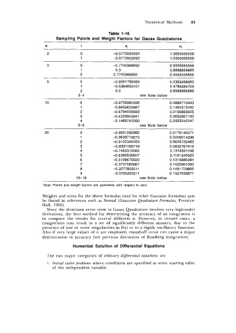
Table 1-16
Sampling Points and Weight Factors for Gauss Quadratures
n i 5 WI
2 0 -0.5773502692 1 .oooooooooo
1 -0.5773502692 1 .oooooooooo
3 0 -0.7745966692 0.5555555556
1 0.0 0.8888888889
2 0.7745966692 0.5555555556
5 0 -0.9061 798459 0.2369268850
1 -0.53846931 01 0.4786286705
2 0.0 0.5688888889
3-4 see Note below
10 0 -0.9739065285 0.066671 3443
1 -0.8650633667 0.149451 3492
2 -0.6794095683 0.21 90863625
3 -0.4333953941 0.26926671 93
4 -0.1 488743390 0.2955242247
5-9 see Note below
20 0 -0.9931 285992 0.0176140071
1 -0.963971 9273 0.040601 4298
2 -0.91 22344283 0.0626720483
3 -0.8391169718 0.083276741 6
4 -0.746331 9065 0.101 93011 98
5 -0.6360536807 0.11 81 945320
6 -0.51 08670020 0.1 31 6886384
7 -0.3737060887 0.1 420961 093
8 -0.227785851 1 0.1491 729865
9 -0.076526521 1 0,1527533871
10-1 9 see Note below
Note: Points and weight factors are symmetric with respect to zero.

Weights and zeros for the above formulas (and for other Gaussian formulas) may
be found in references such as Stroud (Gaussian Quadrature Formulas, Prentice-
Hall, 1966).
Since the dominant error term in Gauss Quadrature involves very high-order
derivatives, the best method for determining the accuracy of an integration is
to compare the results for several different n. However, in certain cases, a
comparison may result in a set of significantly different answers, due to the
presence of one or more singularities in f(x) or to a highly oscillatory function.
Also if very large values of n are employed, round-off error can cause a major
deterioration in accuracy (see previous discussion of Romberg integration)

Numerical Solution of Differential Equations
The two major categories of ordinary differential equations are
1. Initial value problems where conditions are specified at some starting value
of the independent variable.