Page 99 - Standard Handbook Of Petroleum & Natural Gas Engineering

88 Mathematics

3. Corrector

1 3
y p = -(9y, -yi-2)+-Ax(f:;; +2f, -f,-l)
8 8
Truncation error estimates can be made to determine if the step size should be
reduced or increased. For example, for the Hamming method,

The Gear Algorithm [15], based on the Adams formulas, adjusts both the order
and mesh size to produce the desired local truncation error. BuEirsch and Stoer
method [16, 221 is capable of producing accurate solutions using step sizes that
are much smaller than conventional methods. Packaged Fortran subroutines for
both methods are available.
One approach to second-order boundary value probZems is a matrix formulation.
Given

d2Y
-+Ay=B, y(O)=O, y(L)=O
dx2
the function can be represented at i by

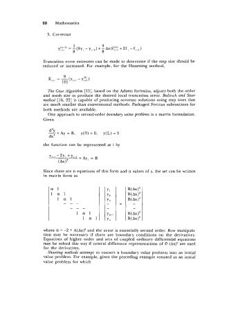
Since there are n equations of this form and n values of y, the set can be written
in matrix form as

a1 YI
1 a1 Y2
1 a1 Y3
--- -
--- -
la1 Y"-1
1 a1 Y,

where a = -2 + A(Ax)~ and the error is essentially second order. Row manipula-
tion may be necessary if there are boundary conditions on the derivatives.
Equations of higher order and sets of coupled ordinary differential equations
may be solved this way if central difference representations of 0 (Ax)' are used
for the derivatives.
Shooting methods attempt to convert a boundary value problem into an initial
value problem. For example, given the preceding example restated as an initial
value problem for which