Page 102 - Standard Handbook Of Petroleum & Natural Gas Engineering

Numerical Methods 91

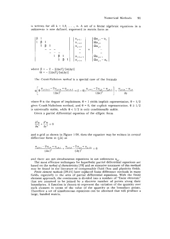
is written for all k = 1,2, . . ., n. A set of n linear algebraic equations in n
unknowns is now defined, expressed in matrix form as

where P = - 2 - [(Ax)*]/[a(Ay)]
Q = - [(Ax)'l/[a(Ay)l

The Crank-Nicholson method is a special case of the formula

where 8 is the degree of implicitness, 8 = 1 yields implicit representation, 8 = 1/2
gives Crank-Nicholson method, and 8 = 0, the explicit representation. 8 2 1/2
is universally stable, while 8 < 1/2 is only conditionally stable.
Given a partial differential equation of the elliptic form

-+-=o
aZu aZU
ax2 ay2

and a grid as shown in Figure 1-58, then the equation may be written in central
difference form at (j,k) as

and there are mn simultaneous equations in mn unknowns u,,!.
The most effective techniques for hyperbolic partial differential equations are
based on the method ofcharacteristics [19] and an extensive treatment of this method
may be found in the literature of compressible fluid flow and plasticity fields.
Finite element methods [20,2 11 have replaced finite difference methods in many
fields, especially in the area of partial differential equations. With the finite
element approach, the continuum is divided into a number of "finite elements"
that are assumed to be joined by a discrete number of points along their
boundaries. A function is chosen to represent the variation of the quantity over
each element in terms of the value of the quantity at the boundary points.
Therefore a set of simultaneous equations can be obtained that will produce a
large, banded matrix.