Page 19 -

6 Monte Carlo methods

butdoes not change the fact that comes outas fourtimes the ratioof
hits to trials.
Those who hear this story for the first time often find it dubious.They
observe that perhaps one shouldnotpile upstones, as in Fig.1.3,if the
aim is to spread them outevenly. This objectionplaces these modern
critics in the illustriouscompanyofprominent physicists and mathe-
maticians whoquestioned the validityofthis method when it was first
published in 1953 (it was applied to the hard-disk system of Chapter 2).
Letters were written, arguments were exchanged, and the issue was set-
tled only after several months. Of course, at the time, helicopters and
heliports were much less common than they are today.
A proof ofcorrectness and an understanding ofthis method, called
the Metropolis algorithm, will follow later, in Subsection 1.1.4.Here,
westart by programming the adults’ algorithm according to the above
prescription: go from one configurationto the nextby followingarandom
throw:
∆ x ← ran (−δ, δ) ,
∆ y ← ran (−δ, δ)
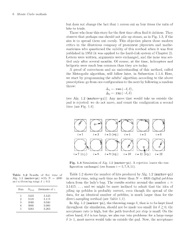
(see Alg.1.2 (markov-pi)). Any movethat wouldtake us outside the
pad is rejected: wedo notmove, and count the configurationa second
time (see Fig.1.4).

i = 1 i = 2 i = 3 (rej.) i = 4 i = 5 i = 6

i = 7 (rej.) i = 8 i = 9 (rej.) i = 10 i = 11 (rej.) i = 12

Fig. 1.4 Simulation of Alg. 1.2 (markov-pi). A rejection leaves the con-
figuration unchanged (see frames i =3, 7, 9, 11).

Table 1.2 Results of five runs of Table 1.2showsthe number ofhits produced byAlg.1.2 (markov-pi)
Alg. 1.2 (markov-pi)with N = 4000 in several runs, using each time no fewer than N = 4000 digital pebbles
and a throwing range δ =0.3 taken fromthe lady’sbag.The results scatter around the number =
3.1415 ... ,and wemight be more inclined to admit that the idea of
Run N hits Estimate of
piling uppebbles is probably correct, even though the spread ofthe
data, foran identical number ofpebbles, is much larger than forthe
1 3123 3.123
2 3118 3.118 direct-sampling method (see Table 1.1).
3 3040 3.040 In Alg.1.2 (markov-pi),the throwing range δ,that isto be kept fixed
4 3066 3.066
5 3263 3.263 throughoutthe simulation, shouldnotbemadetoo small:for δ 0,the
acceptance rate is high, but the path traveled per step is small. On the
other hand, if δ is too large, wealso runinto problems: fora large range
δ 1,most moves wouldtake us outside the pad.Now, the acceptance