Page 21 -

8 Monte Carlo methods

procedure markov-pi(patch)
input {x, y} (configuration i)
∆ x ← ...
∆ y ← ...
.
.
.
output {x, y} (configuration i +1)

Algorithm 1.3 markov-pi(patch). Going from one configuration to the
next, in the Markov-chain Monte Carlo algorithm.

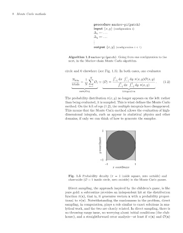
circleand 0 elsewhere (see Fig.1.5). Inboth cases, one evaluates
N 1 1
1 dx dyπ(x, y)O(x, y)
N hits −1 −1
= O i O = . (1.2)
trials N 1 dx 1 dyπ(x, y)
i=1 −1 −1

sampling integration
The probability distribution π(x, y) nolonger appears onthe left: rather
than being evaluated, it is sampled.This is what defines the Monte Carlo
method. On the left ofeqn (1.2),the multipleintegralshave disappeared.
This means that the Monte Carlo methodallowsthe evaluation ofhigh-
dimensional integrals, such as appear in statistical physics and other
domains, if only wecan think ofhow to generate the samples.

1
coordinate

y-

−1
−1 1
x-coordinate

Fig. 1.5 Probability density (π = 1 inside square, zero outside) and
observable (O = 1 inside circle, zero outside) in the Monte Carlo games.

Direct sampling, the approach inspired by the children’s game, is like
pure gold: a subroutine provides an independent hit at the distribution
function π(x), that is, it generates vectors x with a probability propor-
tional to π(x). Notwithstanding the randomness in the problem, direct
sampling, in computation, playsa rolesimilar to exact solutions in ana-
lyticalwork, and the two are closely related.In direct sampling, there is
no throwing-range issue, noworrying aboutinitial conditions (the club-
house), and a straightforward erroranalysis—at least if π(x) and O(x)