Page 232 - Statistics II for Dummies

216 Part III: Analyzing Variance with ANOVA

freedom (n – k and k – 1, respectively, where n is the sample size and k is
the number of treatments) to get the mean sums of squares for error (MSE)
and mean sums of squares for treatment (MST). In general, you want MST to
be large compared to MSE, indicating that the model fits well. The results of
all these statistical gymnastics are summarized by Minitab in a table called
(cleverly) the ANOVA table.

The ANOVA table shown in the bottom part of Figure 12-1 for the Internet use
data example represents the ANOVA table you get from using the regression
line as your model. Under the Source column, you may be used to seeing
treatment, error, and total. For regression, the treatment is the regression
line, so you see regression instead of treatment. The error term in ANOVA is
labeled residual error, because in regression, you measure error in terms of
residuals. Finally you see total, which is the same the world around.

The SS column represents the sums of squares for the regression model. The
three sums of squares listed in the SS column are SSR (for regression), SSE
(for residuals), and SST (total). These sums of squares are calculated using
the formulas from the previous section; the degrees of freedom, DF in the
table, are found by using the formulas from the previous section also.

The MS column takes the value of SS[you fill in the blank] and divides it by
the respective degrees of freedom, just like ANOVA. For example in Figure
12-1, SSE is 12968.5, and the degrees of freedom is 248. Take the first value
divided by the second one to get 52.29 or 52.3, which is listed in the ANOVA
table for MSE.
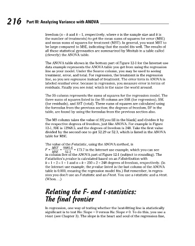
The value of the F-statistic, using the ANOVA method, is
173.7 in the Internet use example, which you can see
in column five of the ANOVA part of Figure 12-1 (subject to rounding). The
F-statistics’s p-value is calculated based on an F-distribution with
k – 1 = 2 – 1 = 1 and n – k = 250 – 2 = 248 degrees of freedom, respectively. (In
the Internet use example, the p-value listed in the last column of the ANOVA
table is 0.000, meaning the regression model fits.) But remember, in regres-
sion you don’t use an F-statistic and an F-test. You use a t-statistic and a t-test.
(Whoa. . .)

Relating the F- and t-statistics:
The final frontier

In regression, one way of testing whether the best-fitting line is statistically
significant is to test Ho: Slope = 0 versus Ha: Slope ≠ 0. To do this, you use a
t-test (see Chapter 3). The slope is the heart and soul of the regression line,

18_466469-ch12.indd 216 7/24/09 9:45:35 AM