Page 202 -

DOMAIN-SPECIFIC & IMPLEMENTATION-INDEPENDENT SOFTWARE ARCHITECTURES 187
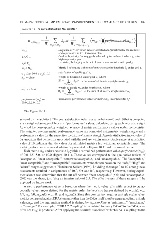
Figure 10.10 Goal Satisfaction Calculation

 
(
σ = ∑ KZ (∑  ) PZ SHUIRUPDQFHP ) 

L J*∈ ' HULY : LM J J + L LM  : L ∀∈ M ∀  P LMN K0∈ LM L K L K L M LMN L MN  

G Deriv Sequence of “Derivation Goals” selected and prioritized by the architect
and represented in the Derivation Plan
g ∈ G Deriv Goal with priority i among goals selected by the architect, where g is the
1
i
highest priority goal
h ∈ H Heuristic j belonging to the set of heuristics associated with goal g i
LM J LM

m ∈ M Metric k belonging to the set of metrics related to heuristic h under goal g
LMN K LM ij i
σ IORDW _ ≤ σ ≤ 10.0 satisfaction of quality goal g i
J L
J
L
h Z IORDW weight of heuristic h under goal g, where
ij
i
LM : L ∑ K = L M Z
LM J L K ∀∈ J + L is the sum of all heuristic weights under g i
m Z IORDW weight of metric m under heuristic h , where
ijk
ij
LMN : LM P = ∑ LMN Z is the sum of all metric weights under h ij

LMN P ∀ L M K ∈ K 0 LM
performance(m ) → normalized performance value for metric m under heuristic h *
ij
ijk
ijk
{0.0,2.5,5.0,10.0}
*See Figure 10.12.
*See Figure 10.11.
2
selected by the architect. The goal satisfaction index is a value between 0 and 10 that is computed
via a weighted average of heuristic “performance” values, calculated using each heuristic weight
h .w and the corresponding weighted average of metric performance values under the heuristic.
ij
The weighted average metric performance values are computed using metric weights m .w and a
ijk
performance value for the respective metric, performance(m ). A goal satisfaction index value of
ijk
0 symbolizes that no metrics associated with the goal are within an acceptable range. A satisfaction
value of 10 indicates that the values for all related metrics fell within an acceptable range. The
metric performance value calculation is presented in Figure 10.11 and discussed below.
Each metric m under a heuristic h yields a normalized performance value, performance(m ),
ij
ijk
ijk
of 0.0, 2.5, 5.0, or 10.0 (Figure 10.11). These values correspond to the qualitative notions of
“ acceptable,” “near acceptable,” “somewhat acceptable,” and “unacceptable.” The “acceptable,”
“near acceptable,” and “unacceptable” assessments were chosen based on the “safe,” “flag,” and
“alarm” ranges suggested in Henderson-Sellers (1996). Dividing the range 0 to 10 among these
assessments resulted in assignments of 10.0, 5.0, and 0.0, respectively. However, during experi-
mentation it was determined that the cut-off between “near acceptable” (5.0) and “unacceptable”
(0.0) was too sharp, justifying an interim value of 2.5. The effectiveness of these ranges will be
explored by future work.
A metric performance value is based on where the metric value falls with respect to the ac-
ceptable value ranges defined for the metric under the heuristic (ranges defined by m .ld2, m .
ijk
ijk
ld1, m .ld0, m .rd0, m .rd1, and m .rd2). Since this comparison requires a single scalar value,
ijk
ijk
ijk
ijk
metrics computed against DRA elements other than the DRA itself must be aggregated into a single
value, a , and the aggregation method is defined by m .sumRule as “minimum,” “maximum,”
ijk
ijk
or “average.” For example, if “DRAC Coupling” is calculated for every DRAC in the DRA, a set
of values (V ) is produced. After applying the sumRule associated with “DRAC Coupling” to the
ijk