Page 123 - The Combined Finite-Discrete Element Method

106 CONTACT DETECTION

Thus, the list for row i y = 6 (i.e. the list y 6 )in Figure 3.41was assembledbyplacing
discrete element 3 onto the list. It is then ‘pushed’ by discrete element 6, which in turn
is ‘pushed’ by discrete element 8, which in turn is ‘pushed’ by discrete element 9, which
was the last discrete element added to the list.
Digital representation of all y-lists (empty and non-empty) is achieved through two
integer arrays. The arrays are common for all the y-lists, and contain enough information
to read all the discrete elements from each of the lists.
The first array B contains the number of the last discrete element mapped to each row,
i.e. the head of the singly connected list for each row of cells. The array B is a 1D array
of size n y ,where n y is the total number of cells in the y direction, i.e. the total number
of rows of cells.
The second array Y is 1D array of size N,where N is the total number of discrete
elements. For each discrete element, the array Y contains the next discrete element in the
singly connected list.
For both arrays a negative number is used as termination of a singly connected list.
So if there are no elements in a particular row, a negative number is assigned to the
corresponding element of the array B.
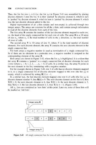
Both arrays are shown in Figure 3.42, where the list y 6 is highlighted. It is evident that
the array B contains a ‘pointer’ to a singly connected list of discrete elements for each
i-row (where i y = 0, 1, 2, 3,..., n y − 1) of cells. In a similar way, the array Y points to
the next element in the list, terminating with a negative number.
For the example shown in Figure 3.40, row 1 of cells has no discrete elements mapped
to it, so a singly connected list of discrete elements mapped to this row (the list y 0 )is
empty, which is achieved by setting B[1] =−1.
In a similar way, the last discrete element mapped onto row 6 of cells (the list y 6 )is
discrete element number 9, thus B[6] = 9. The next discrete element on this list is 8, thus
Y[9] = 8; the next discrete element is 6, thus Y[8] = 6; the next discrete element is 3,
thus Y[6] = 3; the last discrete element is 3, thus Y[3] =−1, (Figure 3.40).
All y iy lists are considered as ‘new lists’ at this point. Later on, some of these lists will
be marked as ‘old lists’.

Integer array B

−1 −1 −1 −1 5 9 10 2 −1 −1

−1 −1 −1 1 −1 3 4 6 8 7

Integer array Y

Figure 3.42 All singly connected lists for rows of cells represented by two arrays.