Page 237 - The Combined Finite-Discrete Element Method

220 SENSITIVITY TO INITIAL CONDITIONS

6.2 COMBINED FINITE-DISCRETE ELEMENT SYSTEMS

The long-term prediction of chaotic system is impossible. In the case of the combined
finite-discrete element method, each body (discrete element) deforms, fractures, fragments
and, at the same time, interacts with discrete elements in its vicinity. Thus, the average
combined finite-discrete element simulation is highly nonlinear.
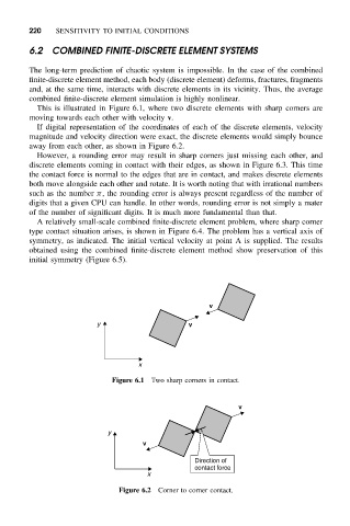
This is illustrated in Figure 6.1, where two discrete elements with sharp corners are
moving towards each other with velocity v.
If digital representation of the coordinates of each of the discrete elements, velocity
magnitude and velocity direction were exact, the discrete elements would simply bounce
away from each other, as shown in Figure 6.2.
However, a rounding error may result in sharp corners just missing each other, and
discrete elements coming in contact with their edges, as shown in Figure 6.3. This time
the contact force is normal to the edges that are in contact, and makes discrete elements
both move alongside each other and rotate. It is worth noting that with irrational numbers
such as the number π, the rounding error is always present regardless of the number of
digits that a given CPU can handle. In other words, rounding error is not simply a mater
of the number of significant digits. It is much more fundamental than that.
A relatively small-scale combined finite-discrete element problem, where sharp corner
type contact situation arises, is shown in Figure 6.4. The problem has a vertical axis of
symmetry, as indicated. The initial vertical velocity at point A is supplied. The results
obtained using the combined finite-discrete element method show preservation of this
initial symmetry (Figure 6.5).

v

y v

x

Figure 6.1 Two sharp corners in contact.

v

y
v
Direction of
contact force
x
Figure 6.2 Corner to corner contact.