Page 49 - The Combined Finite-Discrete Element Method

32 INTRODUCTION

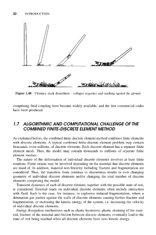
Figure 1.48 Chimney stack demolition – collapse sequence and crashing against the ground.

comprising fluid coupling have become widely available, and the first commercial codes
have been produced.

1.7 ALGORITHMIC AND COMPUTATIONAL CHALLENGE OF THE
COMBINED FINITE-DISCRETE ELEMENT METHOD

As explained before, the combined finite discrete element method combines finite elements
with discrete elements. A typical combined finite-discrete element problem may contain
thousands, even millions, of discrete elements. Each discrete element has a separate finite
element mesh. Thus, the model may contain thousands to millions of separate finite
element meshes.
The nature of the deformation of individual discrete elements involves at least finite
rotations. Finite strains may be involved depending on the material that discrete elements
are maid of. In addition, material non-linearity including fracture and fragmentation are
considered. Thus, the transition from continua to discontinua results in ever changing
geometry of individual discrete elements and/or changing the total number of discrete
elements comprising the model.
Transient dynamics of each of discrete element, together with the possible state of rest,
is considered. External loads on individual discrete elements often include interaction
with fluid. Such is the case, for instance, in explosive induced fragmentation, where a
detonation gas pushes against the walls of discrete elements causing further fracture and
fragmentation, or increasing the kinetic energy of the system, i.e. increasing the velocity
of individual discrete elements.
Energy dissipation mechanisms such as elastic hysteresis, plastic straining of the mate-
rial, fracture of the material and friction between discrete elements, eventually lead to the
state of rest being reached when all discrete elements have zero kinetic energy.