Page 359 - The Mechatronics Handbook

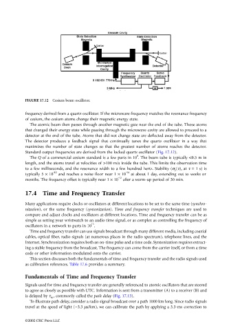
FIGURE 17.12 Cesium beam oscillator.

frequency derived from a quartz oscillator. If the microwave frequency matches the resonance frequency
of cesium, the cesium atoms change their magnetic energy state.
The atomic beam then passes through another magnetic gate near the end of the tube. Those atoms
that changed their energy state while passing through the microwave cavity are allowed to proceed to a
detector at the end of the tube. Atoms that did not change state are deflected away from the detector.
The detector produces a feedback signal that continually tunes the quartz oscillator in a way that
maximizes the number of state changes so that the greatest number of atoms reaches the detector.
Standard output frequencies are derived from the locked quartz oscillator (Fig. 17.12).
8
The Q of a commercial cesium standard is a few parts in 10 . The beam tube is typically <0.5 m in
length, and the atoms travel at velocities of >100 m/s inside the tube. This limits the observation time
to a few milliseconds, and the resonance width to a few hundred hertz. Stability (σ y (τ), at τ = 1 s) is
-14
-12
typically 5 × 10 and reaches a noise floor near 1 × 10 at about 1 day, extending out to weeks or
-12
months. The frequency offset is typically near 1 × 10 after a warm-up period of 30 min.
17.4 Time and Frequency Transfer

Many applications require clocks or oscillators at different locations to be set to the same time (synchro-
nization), or the same frequency (syntonization). Time and frequency transfer techniques are used to
compare and adjust clocks and oscillators at different locations. Time and frequency transfer can be as
simple as setting your wristwatch to an audio time signal, or as complex as controlling the frequency of
13
oscillators in a network to parts in 10 .
Time and frequency transfer can use signals broadcast through many different media, including coaxial
cables, optical fiber, radio signals (at numerous places in the radio spectrum), telephone lines, and the
Internet. Synchronization requires both an on-time pulse and a time code. Syntonization requires extract-
ing a stable frequency from the broadcast. The frequency can come from the carrier itself, or from a time
code or other information modulated onto the carrier.
This section discusses both the fundamentals of time and frequency transfer and the radio signals used
as calibration references. Table 17.6 provides a summary.

Fundamentals of Time and Frequency Transfer
Signals used for time and frequency transfer are generally referenced to atomic oscillators that are steered
to agree as closely as possible with UTC. Information is sent from a transmitter (A) to a receiver (B) and
is delayed by τ ab , commonly called the path delay (Fig. 17.13).
To illustrate path delay, consider a radio signal broadcast over a path 1000 km long. Since radio signals
travel at the speed of light (~3.3 µs/km), we can calibrate the path by applying a 3.3-ms correction to

©2002 CRC Press LLC