Page 354 - The Mechatronics Handbook

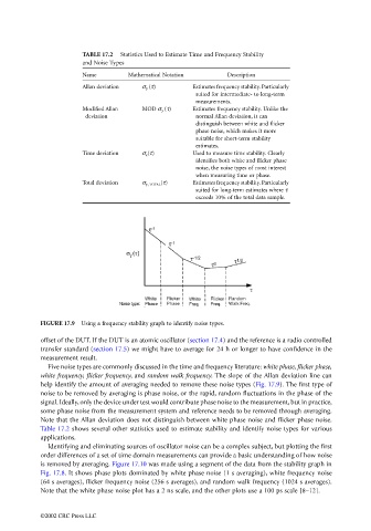
TABLE 17.2 Statistics Used to Estimate Time and Frequency Stability
and Noise Types
Name Mathematical Notation Description
Allan deviation σ γ (τ) Estimates frequency stability. Particularly
suited for intermediate- to long-term
measurements.
Modified Allan MOD σ γ (τ) Estimates frequency stability. Unlike the
deviation normal Allan deviation, it can
distinguish between white and flicker
phase noise, which makes it more
suitable for short-term stability
estimates.
Time deviation σ x (τ) Used to measure time stability. Clearly
identifies both white and flicker phase
noise, the noise types of most interest
when measuring time or phase.
Total deviation σ γ ,TOTAL (τ) Estimates frequency stability. Particularly
suited for long-term estimates where τ
exceeds 10% of the total data sample.

FIGURE 17.9 Using a frequency stability graph to identify noise types.

offset of the DUT. If the DUT is an atomic oscillator (section 17.4) and the reference is a radio controlled
transfer standard (section 17.5) we might have to average for 24 h or longer to have confidence in the
measurement result.
Five noise types are commonly discussed in the time and frequency literature: white phase, flicker phase,
white frequency, flicker frequency, and random walk frequency. The slope of the Allan deviation line can
help identify the amount of averaging needed to remove these noise types (Fig. 17.9). The first type of
noise to be removed by averaging is phase noise, or the rapid, random fluctuations in the phase of the
signal. Ideally, only the device under test would contribute phase noise to the measurement, but in practice,
some phase noise from the measurement system and reference needs to be removed through averaging.
Note that the Allan deviation does not distinguish between white phase noise and flicker phase noise.
Table 17.2 shows several other statistics used to estimate stability and identify noise types for various
applications.
Identifying and eliminating sources of oscillator noise can be a complex subject, but plotting the first
order differences of a set of time domain measurements can provide a basic understanding of how noise
is removed by averaging. Figure 17.10 was made using a segment of the data from the stability graph in
Fig. 17.8. It shows phase plots dominated by white phase noise (1 s averaging), white frequency noise
(64 s averages), flicker frequency noise (256 s averages), and random walk frequency (1024 s averages).
Note that the white phase noise plot has a 2 ns scale, and the other plots use a 100 ps scale [8–12].

©2002 CRC Press LLC