Page 353 - The Mechatronics Handbook

works with stationary data, where the results are time independent, and the noise is white, meaning that
it is evenly distributed across the frequency band of the measurement. Oscillator data is usually nonsta-
tionary, since it contains time dependent noise contributed by the frequency offset. With stationary data,
the mean and standard deviation will converge to particular values as more measurements are made.
With nonstationary data, the mean and standard deviation never converge to any particular values.
Instead, there is a moving mean that changes each time we add a measurement.
For these reasons, a non-classical statistic is often used to estimate stability in the time domain. This
statistic is sometimes called the Allan variance, but since it is the square root of the variance, its proper
name is the Allan deviation. The equation for the Allan deviation (σ y (τ)) is

M-1
1 ( ∑ 2
σ y τ() = ---------------------- y i+1 – )
(
2 M 1)
–
y i
i=1
where y i is a set of frequency offset measurements containing y 1 , y 2 , y 3 , and so on, M is the number of
values in the y i series, and the data are equally spaced in segments τ seconds long. Or
N-2
1 2∑ 2
σ y τ() = -------------------------- [ x i+2 – 2x i+1 + ]
x i
–
(
2 N 2)τ i=1
where x i is a set of phase measurements in time units containing x 1 , x 2 , x 3 , and so on, N is the number
of values in the x i series, and the data are equally spaced in segments τ seconds long. Note that while
standard deviation subtracts the mean from each measurement before squaring their summation, the
Allan deviation subtracts the previous data point. This differencing of successive data points removes
the time dependent noise contributed by the frequency offset.
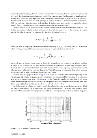
An Allan deviation graph is shown in Fig. 17.8. It shows the stability of the device improving as the
averaging period (τ) gets longer, since some noise types can be removed by averaging. At some point,
however, more averaging no longer improves the results. This point is called the noise floor, or the point
where the remaining noise consists of nonstationary processes such as flicker noise or random walk. The
-11
device measured in Fig. 17.8 has a noise floor of ~5 × 10 at τ = 100 s.
Practically speaking, a frequency stability graph also tells us how long we need to average to get rid of
the noise contributed by the reference and the measurement system. The noise floor provides some
indication of the amount of averaging required to obtain a TUR high enough to show us the true frequency

FIGURE 17.8 A frequency stability graph.

©2002 CRC Press LLC