Page 973 - The Mechatronics Handbook

0066_Frame_C32.fm Page 23 Wednesday, January 9, 2002 7:54 PM

DRY NORMAL WET
COLD M S S
COOL M M S
WARM L M S
HOT L M S
(a)
DRY NORMAL WET
0 0.4 0.6
COLD 0 0 0 0
COOL 0.2 0 0.2 0.2
WARM 0.5 0 0.4 0.5
HOT 0 0 0 0
(b)

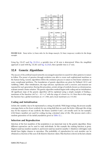
FIGURE 32.24 Fuzzy tables: (a) fuzzy rules for the design example, (b) fuzzy temporary variables for the design
example.

Using Eq. (32.47) and Fig. 32.23(c), a sprinkle time of 28 min is determined. When the simplified
approach is used with Eq. (32.46) and Fig. 32.23(d), then sprinkle time is 27 min.

32.8 Genetic Algorithms

The success of the artificial neural networks encouraged researchers to search for other patterns in nature
to follow. The power of genetics through evolution was able to create such sophisticated machines as
the human being. Genetic algorithms follow the evolution process in nature to find better solutions to
some complicated problems. The foundations of genetic algorithms are given by Holland (1975) and
Goldberg (1989). After initialization, the steps selection, reproduction with a crossover, and mutation are
repeated for each generation. During this procedure, certain strings of symbols, known as chromosomes,
evaluate toward a better solution. The genetic algorithm method begins with coding and an initialization.
All significant steps of the genetic algorithm will be explained using a simple example of finding a
2
2
maximum of the function (sin (x) − 0.5 ∗ x) with the range of x from 0 to 1.6. Note that in this range,
the function has a global maximum at x = 1.309, and a local maximum at x = 0.262.
Coding and Initialization
At first, the variable x has to be represented as a string of symbols. With longer strings, the process usually
converges faster, so the fewer symbols for one string field that are used, the better. Although this string
may be the sequence of any symbols, the binary symbols 0 and 1 are usually used. In our example,
6-bit binary numbers are used for coding, having a decimal value of 40x. The process starts with a
random generation of the initial population given in Table 32.1.

Selection and Reproduction
Selection of the best members of the population is an important step in the genetic algorithm. Many
different approaches can be used to rank individuals. In this example the ranking function is given.
Highest rank has member number 6, and lowest rank has member number 3. Members with higher rank
should have higher chances to reproduce. The probability of reproduction for each member can be
obtained as a fraction of the sum of all objective function values. This fraction is shown in the last column

©2002 CRC Press LLC