Page 111 - Thomson, William Tyrrell-Theory of Vibration with Applications-Taylor _ Francis (2010)

98 Transient Vibration Chap. 4

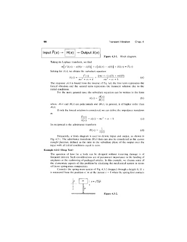
Input F (s ) H (s) Output x ( s )
Figure 4.3-1. Block diagram.
Taking its Laplace transform, we find
m\^s^x{s) — x(0).9 - i(0 )] + c[5x(5) - x(0 )] + kx{s) = F(s)
Solving for xC^), we obtain the subsidiary equation:
n o (ms + c)x(O) + mi(0)
x{s) = (a)
ms^ cs k ms^ + cs + k
The response x(t) is found from the inverse of Eq. (a); the first term represents the
forced vibration and the second term represents the transient solution due to the
initial conditions.
For the more general case, the subsidiary equation can be written in the form

x(i) = (b)
B(s)
where A(s) and B(s) are polynomials and B(s), in general, is of higher order than
^ (5).
If only the forced solution is considered, we can define the impedance transform
as
F{s)
= 2 ( 5 ) = ms^ + cs + k (c)
x{s)
Its reciprocal is the admittance transform

His) - (d)
z{s)
Frequently, a block diagram is used to denote input and output, as shown in
Fig. 4.3-1. The admittance transform H(s) then can also be considered as the system
transfer function, defined as the ratio in the subsidiary plane of the output over the
input with all initial conditions equal to zero.
Example 4.3-2 (Drop Test)
The question of how far a body can be dropped without incurring damage is of
frequent interest. Such considerations are of paramount importance in the landing of
airplanes or the cushioning of packaged articles. In this example, we discuss some of
the elementary aspects of this problem by idealizing the mechanical system in terms
of linear spring-mass components.
Consider the spring-mass system of Fig. 4.3-2 dropped through a height h. If x
is measured from the position of m at the instant t = 0 when the spring first contacts

X = y 2 g h

y/77777/7/7? Figure 4.3-2.