Page 126 - Thomson, William Tyrrell-Theory of Vibration with Applications-Taylor _ Francis (2010)

Sec. 4.7 Finite Difference Numerical Computation 113

forces. The equations to be superimposed for the exact solution are
jCj = 0.05(1 —cos22.36r) 0 < / < 0.1

•«2 = - [ i ( i - 0.1) - 0.02236sin 22.36(; - 0.10)] add at t = 0.1

•»^3= + P ( < - 0.2) - 0.02236sin22.36(t - 0.2)] add at t = 0.2
Both computations were carried out on a programmable hand calculator.
Initial acceleration and initial conditions zero. If the applied force is
zero at r = 0 and the initial conditions are zero, will also be zero and the
computation cannot be started because Eq. (4.7-8) gives X2 = 0. This condition can
be rectified by developing new starting equations based on the assumption that
during the first-time interval the acceleration varies linearly from x^ = 0 to T’2
follows:
X = 0 at
Integrating, we obtain
a y
x =
a y
X - -g-r
Because from the first equation, Xy = ah, where h = Ar, the second and third
equations become
(4.7-9)

(4.7-10)
6 -^2
Substituting these equations into the differential equation at time ty = h enables
one to solve for Xy and Xy. Example 4.7-2 illustrates the situation encountered
here.
Example 4.7-2
Use the digital computer to solve the problem of a spring-mass system excited by a
triangular pulse. The differential equation of motion and the initial conditions are
given as
0.5jc -h = F{t)
j
jC = ij = 0
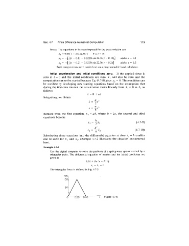
The triangular force is defined in Fig. 4.7-5.

Figure 4.7-5.