Page 124 - Thomson, William Tyrrell-Theory of Vibration with Applications-Taylor _ Francis (2010)

Sec. 4.7 Finite Difference Numerical Computation 111

Thus, Eq. (4.7-8) enables one to find X2 in terms of the initial conditions, after
which X3, X4, ... are available from Eq. (4.7-7).
In this development we have ignored higher-order terms that introduce what
is known as truncation errors. Other errors, such as round-off errors, are intro­
duced due to loss of significant figures. These are all related to the time increment
h = At in a rather complicated way, which is beyond the scope of this text. In
general, better accuracy is obtained by choosing a smaller but the number of
computations will then increase together with errors generated in the computation.
A safe rule to use in Method 1 is to choose h < r/10, where r is the natural
period of the system.
A flow diagram for the digital calculation is shown in Fig. 4.7-1. From the
given data in block we proceed to block (S), which is the differential
equation. Going to © for the first time, I is not greater than 1, and hence we
proceed to the left, where ^2 is calculated. Increasing / by 1, we complete the left
loop © and © , where / is now equal to 2, so we proceed to the right to
calculate JC3. Assuming N intervals of At, the path is to the No direction and the
right loop is repeated N times until I = N 1, at which time the results are
printed out.
Example 4.7-1
Solve numerically the differential equation
4x + 2000 jc = F(t)
with initial conditions
Xj = ij = 0
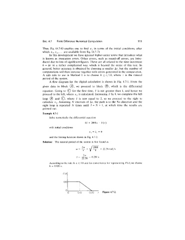
and the forcing function shown in Fig. 4.7-2.
Solution: The natural period of the system is first found as
I tt [ 2000

o>= — = y = 22.36 rad/s
4
277
2236 0.281 s
According to the rule h < r/10 and for convenience for representing F(t), we choose
h = 0.020 s.

Figure 4.7-2.