Page 132 - Thomson, William Tyrrell-Theory of Vibration with Applications-Taylor _ Francis (2010)

Sec. 4.8 Runge-Kutta Method 119

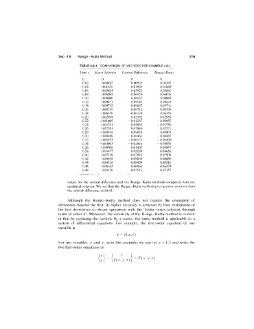
TABLE 4.8-1 COMPARISON OF METHODS FOR EXAMPLE 4.8-1
Time t Exact Solution Central Difference Runge-Kutta
0 0 0 0
0.02 0.00492 0.00500 0.00492
0.04 0.01870 0.01900 0.01869
0.06 0.03864 0.03920 0.03862
0.08 0.06082 0.06159 0.06076
0.10 0.08086 0.08167 0.08083
0.12 0.09451 0.09541 0.09447
0.14 0.09743 0.09807 0.09741
0.16 0.08710 0.08712 0.08709
0.18 0.06356 0.06274 0.06359
0.20 0.02949 0.02782 0.02956
0.22 -0.01005 -0.01267 -0.00955
0.24 -0.04761 - 0.05063 -0.04750
0.26 -0.07581 -0.07846 -0.07571
0.28 -0.08910 -0.09059 -0.08903
0.30 -0.08486 -0.08461 -0.08485
0.32 -0.06393 -0.06171 -0.06400
0.34 -0.03043 - 0.02646 -0.03056
0.36 0.00906 0.01407 0.00887
0.38 0.04677 0.05180 0.04656
0.40 0.07528 0.07916 0.07509
0.42 0.08898 0.09069 0.08886
0.44 0.08518 0.08409 0.08516
0.46 0.06463 0.06066 0.06473
0.48 0.03136 0.02511 0.03157

values for the central difference and the Runge-Kutta methods compared with the
analytical solution. We see that the Runge-Kutta method gives greater accuracy than
the central difference method.

Although the Runge-Kutta method does not require the evaluation of
derivatives beyond the first, its higher accuracy is achieved by four evaluations of
the first derivatives to obtain agreement with the Taylor series solution through
terms of order h‘^. Moreover, the versatility of the Runge-Kutta method is evident
in that by replacing the variable by a vector, the same method is applicable to a
system of differential equations. For example, the first-order equation of one
variable is
i =f { x , t )

For two variables, x and y, as in this example, we can let 2 = {') and write the
two first-order equations as

= F ( x , y j )