Page 144 - Thomson, William Tyrrell-Theory of Vibration with Applications-Taylor _ Francis (2010)

Sec. 5.1 The Normal Mode Analysis 131

multi-DOF system can be described in terms of the 2-DOF system without
becoming burdened with the algebraic difficulties of the multi-DOF system.
Numerical results are easily obtained for the 2-DOF system and they provide a
simple introduction to the behavior of systems of higher DOF.
For systems of higher DOF, matrix methods are essential, and although they
are not necessary for the 2-DOF system, we introduce them here as a preliminary
to the material in the chapters to follow. They provide a compact notation and an
organized procedure for their analysis and solution. For systems of DOF higher
than 2, computers are necessary. A few examples of systems of higher DOF are
introduced near the end of the chapter to illustrate some of the computational
difficulties.

5.1 THE NORMAL MODE ANALYSIS

We now describe the basic method of determining the normal modes of vibration
for any system by means of specific examples. The method is applicable to all
multi-DOF systems, although for systems of higher-DOF, there are more efficient
methods, which we will describe in later chapters.
Example 5.1-1 Translational System
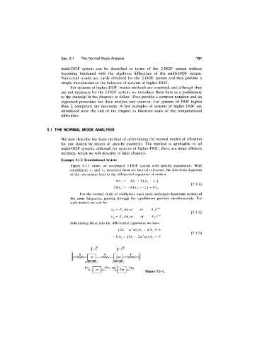
Figure 5.1-1 shows an undamped 2-DOF system with specific parameters. With
coordinates Xj and X2 measured from the inertial reference, the free-body diagrams
of the two masses lead to the differential equations of motion:

mjCj = -/cjCj -h k(x2 —Xj)
(5.1-1)
2mx2 = -k(x2 Xj) —kx2
-

For the normal mode of oscillation, each mass undergoes harmonic motion of
the same frequency, passing through the equilibrium position simultaneously. For
such motion, we can let
x^=A^s\ncot or
(5.1-2)
X2 = A 2^\n (x)t or A2e'"^^
Substituting these into the differential equations, we have
{2k - (o^m)A] - kA2 = 0
(5.1-3)

—kA^ -t- {2k —2oj^m)A2 = 0

k k /
m 2 m /

kX‘^ k{x^-X2) kX2
2 m
Figure 5.1-1.