Page 152 - Thomson, William Tyrrell-Theory of Vibration with Applications-Taylor _ Francis (2010)

Sec. 5.3 Coordinate Coupling 139

or U, The choice of coordinates establishes the type of coupling, and both dynamic
and static coupling may be present.
It is possible to find a coordinate system that has neither form of coupling.
The two equations are then decoupled and each equation can be solved indepen­
dently of the other. Such coordinates are called principal coordinates (also called
normal coordinates).
Although it is always possible to decouple the equations of motion for the
undamped system, this is not always the case for a damped system. The following
matrix equations show a system that has zero dynamic and static coupling, but the
coordinates are coupled by the damping matrix.
m,. 0 0 ■
(M. C| 1 ^12 (M. ^11 (5.3-3)
0 ni22 /■2I ^22 (->2/ 0 ^22
If in the foregoing equation, c,2 = Cjx = 0, then the damping is said to be
proportional (to the stiffness or mass matrix), and the system equations become
uncoupled.
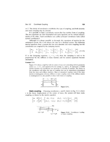
Example 5.3-1
Figure 5.3-1 shows a rigid bar with its center of mass not coinciding with its geometric
system, because two coordinates are necessary to describe its motion. The choice of
the coordinates will define the type of coupling that can be immediately determined
from the mass and stiffness matrices. Mass or dynamical coupling exists if the mass
matrix is nondiagonal, whereas stiffness or static coupling exists if the stiffness matrix
is nondiagonal. It is also possible to have both forms of coupling.

Figure 5.3-1.

Static coupling. Choosing coordinates x and 9, shown in Fig. 5.3-2, where
X is the linear displacement of the center of mass, the system will have static
coupling, as shown by the matrix equation
m 0 (/c, +k2) ( k 2 i 2 - k , i , y
0 J i C (^2^2 ~ ^ 1^1) { k y ^ k 2 l l ) _

Ref.

Figure 5.3-2. Coordinates leading
k2ix + IpO) to static coupling.