Page 153 - Thomson, William Tyrrell-Theory of Vibration with Applications-Taylor _ Francis (2010)

140 Systems with Two or More Degrees of Freedom Chap. 5

M l Z Î

n-fin k:(Xc~l^e)

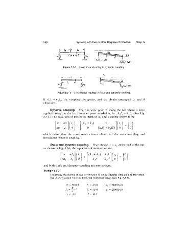
Figure 5.3-3. Coordinates leading to dynamic coupling.

h I-
= l
il' U2(^1

Figure 5.3-4. Coordinates leading to static and dynamic coupling.

If /cj/, = ^ 2^2’ coupling disappears, and we obtain uncoupled x and 6
vibrations.

Dynamic coupling. There is some point C along the bar where a force
applied normal to the bar produces pure translation; i.e., ^ 2^4*
5.3-3.) The equations of motion in terms of and 6 can be shown to be

m me ("•)+ [ ( /c j + /C2 ) 0
me 1 «) [ 0 { k j j + k ,li) e

which shows that the coordinates chosen eliminated the static coupling and
introduced dynamic coupling.

Static and dynamic coupling. If we choose x = at the end of the bar,
as shown in Fig. 5.3-4, the equations of motion become

m ml^ (^1 + ^ 2) k^l ■
P . : U
mi^ y, k^l e
and both static and dynamic coupling are now present.
Example 5.3-2
Determine the normal modes of vibration of an automobile simulated by the simpli-
hed 2-DOF system with the following numerical values (see Fig. 5.3-5):

IT = 3220 lb L = 4.5 ft k^ = 2400 Ib/ft
^ 2
,
T. = —r ^2 = 2600 Ib/ft
^ g
r = 4Ü / = 10 ft