Page 271 - Thomson, William Tyrrell-Theory of Vibration with Applications-Taylor _ Francis (2010)

258 Computational Methods Chap. 8

;d to 1.0,

■-0 .9 4 0 0.225 0.259'
-0.045 0.707 -0 .8 7 2 from
1.00 1.00 1.00
mode 2 mode 1 mode 3
-1 .0 0.25 0.25'
0 0.79 -0 .7 9 from the computer
1.00 1.00 1.00

Cho I esk I - Jacob I Program A = (o^m /k Cho I msk I -Jacob i Program A = k /cj^m
Matrix IM3 Matrix [K1
4000E+01 .OOOOE-i-00 .OOOOE+00 4000E+01 1000E+01 .OOOOE-HX)
OOOOE+00 TOOOE+Oi nnooE-t-00 - IOCiOE+01 2000E+01 - 1000E+01
.OOOOE+00 .OOOOE+00 . 10CWE+01 .OOOOE+00 '.1000E+01 . lOOOE^OI
Matrix [KJ Matrix IM)
4000E+01 1000E+01 .OOOOE+00 4000E+01 OOOOE+00 .OOOOE+00
1000E+01 .2000E+01 . 1000E+01 OOOOE-KX) .2000E+01 ■ OOOOE+00
OOOOE+00 - 1000E+01 1000E+01 OOOOE+00 OOOOE-i'OO 1000E+01
0*jnamic matrix [fl] Dynamic matrix CRl
. 1000E+01 -3536E+00 .OOOOE-fOO . lOOOE+01 378CE+00 .4364E+00
- .3536E+00 . 1000E+01 7071E+00 3780E+00 . 1286E+0I . 1485E+01
OOOCE+00 -.7071E+00 . 1000E+01 •4364E+00 . 1485E+01 .4048E-i'01
Eigmnoaliws arc: Eigenvalues ore;
1791E+01 . 1000E^•01 .2094E+00 .4775E+01 IOOOE‘t'01 .5585E+00
Eigenvectors of Ifll are; Eigenvectors of [R] are:
3162E+00 .8944E+00 .3162E+00 . 1447E+00 -.8944E+00 .4233E+00
-.7071E+00 .2551E-05 .7071E+00 .4006E+00 -.3382E+00 .8515E+00
6325E+00 - 4472E+00 6324E-^00 9047E-MX) 2928E-^00 3094E+00
Rctual eigenvectors are; Rctual eigenvectors are;
1925E+00 - 7071E+00 1924E+00 1925E+00 - 7070E-HD0 1926E-K)0
-.6086E+00 -.2852E-05 .6086E+00 .6086E'»'00 -.5306E-04 .6086E‘i’00
.7698E-I-00 .7071E+00 .7698E-K)0 .7698E+00 .7072E+00 .7698E+00
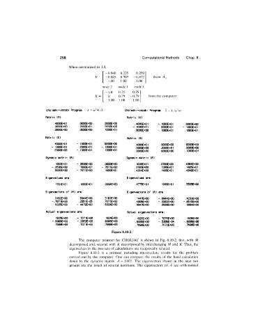
Figure 8.10-2.

The computer printout for CHOLJAC is shown in Fig. 8.10-2, first, with M
decomposed and, second, with K decomposed by interchanging M and K. Thus, the
eigenvalues in the two sets of calculations are reciprocally related.
Figure 8.10-3 is a printout including intermediate results for the problem
carried out by the computer. One can compare the results of the hand calculation
down to the dynamic matrix A = UKU. The eigenvectors shown in the next two
groups are the result of several iterations. The eigenvectors of A are orthonomial