Page 408 - Thomson, William Tyrrell-Theory of Vibration with Applications-Taylor _ Francis (2010)

Sec. 12.6 Mykiestad’s Method for Beams 395

where b¿ are constants and 6^ is unknown. Thus, the frequencies that satisfy the
boundary condition 6^ = = 0 for the cantilever beam will establish 0^ and the
natural frequencies of the beam, i.e., = “ <^3/^3 and - {a2,/b^)b^ = 0.
Hence, by plotting y^ versus w, the natural frequencies of the beam can be found.
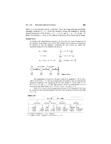
Example 12.6-1
To illustrate the computational procedure, we determine the natural frequencies of
the cantilever beam shown in Fig. 12.6-2. The massless beam sections are assumed to
be identical so that the influence coefficients for each section are equal. The
numerical constants for the problem are given as

mj = 100 kg - ^ = 5 X 10
El Nm
/ = 0.5 m = 1.25 X 10^'’ ITT
2EI N
El = 0.10 X 10~^ N • m^ = 0.41666 X 10“'’^

/7?i ^2 1.5^^ m3 = 2.0m^

■ M >

© © © Figure 12.6-2.

The computation is started at 1. Because each of the quantities K, M, 6, and y
will be in the form a b, they are arranged into two columns, each of which can be
computed separately. The calculation for the left column is started with Fj = 0,
Mj = 0, öj = 0, and y^ = 1.0. The right columns, which are proportional to 6, are
started with the initial values of Fj = 0, Mj = 0, = 10, and = 0.
Table 12.6-1 shows how the computation for Eqs. (12.6-1) through (12.6-4) can
be carried out with any programmable calculator. The frequency chosen for this table
is oj = 10.
TABLE 12.6-1
n = 10. = 100.
F M 0 y
/ (newtons) (newton • meters) (Radians) (meters)
1 0 0 0 0 0 0 1.0 0
2 -10,000. 0 5000. 0 0.0125 1.00 1.002084 0.50
3 -25031. -75000 17515. 37500 0.06879 1.009370 1.0198 1.0015630
4 -45427. -275320 40228. 175160 0.21315 1.06250 1.08555 1.51670
04 = 0.21315 -f 1.06250 = 0 0j = -0.2006117
^4 = 1.08555+ 1.5167C-0.2006117)= 0.78128 plot vs. a; = 10