Page 65 - Thomson, William Tyrrell-Theory of Vibration with Applications-Taylor _ Francis (2010)

52 Harmonically Excited Vibration Chap. 3

Fn sin cot

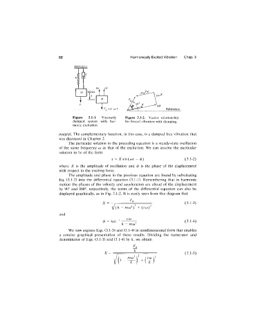
Figure 3.1-1 Viscously Figure 3.1-2. Vector relationship
damped system with har­ for forced vibration with damping.
monic excitation.

integral. The complementary function, in this case, is a damped free vibration that
was discussed in Chapter 2.
The particular solution to the preceding equation is a steady-state oscillation
of the same frequency co as that of the excitation. We can assume the particular
solution to be of the form
X = X - (¡)) (3.1-2)
where X is the amplitude of oscillation and cf) is the phase of the displacement
with respect to the exciting force.
The amplitude and phase in the previous equation are found by substituting
Eq. (3.1-2) into the differential equation (3.1-1). Remembering that in harmonic
motion the phases of the velocity and acceleration are ahead of the displacement
by 90° and 180°, respectively, the terms of the differential equation can also be
displayed graphically, as in Fig. 3.1-2. It is easily seen from this diagram that

= (3.1-3)

{k —mco^) + {ciüŸ
and
CO)

<>= tan ' ---------- j (3.1-4)
f
k —mco

We now express Eqs. (3.1-3) and (3.1-4) in nondimensional form that enables
a concise graphical presentation of these results. Dividing the numerator and
denominator of Eqs. (3.1-3) and (3.1-4) by /c, we obtain
= (3.1-5)
mo)^
{ coj Ÿ
[^
V(>-— ) Mt )