Page 293 - Thermal Hydraulics Aspects of Liquid Metal Cooled Nuclear Reactors

Large-eddy simulation: Application to liquid metal fluid flow and heat transfer 263

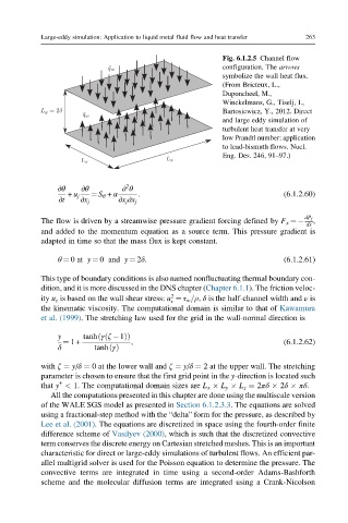
Fig. 6.1.2.5 Channel flow
configuration. The arrows
symbolize the wall heat flux.
(From Bricteux, L.,
Duponcheel, M.,
Winckelmans, G., Tiselj, I.,
Bartosiewicz, Y., 2012. Direct
and large eddy simulation of
turbulent heat transfer at very
low Prandtl number: application
to lead-bismuth flows. Nucl.
Eng. Des. 246, 91–97.)

∂θ ∂θ ∂ θ
2
+ u j ¼ S θ + α : (6.1.2.60)
∂t ∂x j ∂x j ∂x j

dP f
The flow is driven by a streamwise pressure gradient forcing defined by F x ¼ ,
dx
and added to the momentum equation as a source term. This pressure gradient is
adapted in time so that the mass flux is kept constant.
θ ¼ 0at y ¼ 0 and y ¼ 2δ: (6.1.2.61)

This type of boundary conditions is also named nonfluctuating thermal boundary con-
dition, and it is more discussed in the DNS chapter (Chapter 6.1.1). The friction veloc-
2
ity u τ is based on the wall shear stress: u ¼ τ w =ρ, δ is the half-channel width and ν is
τ
the kinematic viscosity. The computational domain is similar to that of Kawamura
et al. (1999). The stretching law used for the grid in the wall-normal direction is
y tanhðγðζ 1ÞÞ
¼ 1+ , (6.1.2.62)
δ tanhðγÞ
with ζ ¼ y/δ ¼ 0 at the lower wall and ζ ¼ y/δ ¼ 2 at the upper wall. The stretching
parameter is chosen to ensure that the first grid point in the y-direction is located such
+
that y < 1. The computational domain sizes are L x L y L z ¼ 2πδ 2δ πδ.
All the computations presented in this chapter are done using the multiscale version
of the WALE SGS model as presented in Section 6.1.2.3.3. The equations are solved
using a fractional-step method with the “delta” form for the pressure, as described by
Lee et al. (2001). The equations are discretized in space using the fourth-order finite
difference scheme of Vasilyev (2000), which is such that the discretized convective
term conserves the discrete energy on Cartesian stretched meshes. This is an important
characteristic for direct or large-eddy simulations of turbulent flows. An efficient par-
allel multigrid solver is used for the Poisson equation to determine the pressure. The
convective terms are integrated in time using a second-order Adams-Bashforth
scheme and the molecular diffusion terms are integrated using a Crank-Nicolson