Page 172 - Bird R.B. Transport phenomena

156 Chapter 5 Velocity Distributions in Turbulent Flow

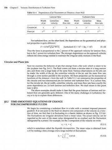
Table 5.1-1 Dependence of Jet Parameters on Distance z from Wall
Laminar flow Turbulent flow

Width Centerline Mass Width Centerline Mass
of jet velocity flow rate of jet velocity flow rate

Circular jet z z" 1 z z z" 1 z
Plane jet z 2/3 z -l/3 z l/3 z z" 1/2 2 1 / 2

For turbulent flow, on the other hand, the dependence on the geometrical and phys-
ical properties is quite different: 1
L W vl (turbulent) (5 X 10 5 < Re < 10 ) (5.1-8)
7
5
4
L
Thus the force is proportional to the |-power of the approach velocity for laminar flow,
but to the |-power for turbulent flow. The stronger dependence on the approach velocity
reflects the extra energy needed to maintain the irregular eddy motions in the fluid.
Circular and Plane Jets
Next we examine the behavior of jets that emerge from a flat wall, which is taken to be
the xy-plane (see Fig. 5.6-1). The fluid comes out from a circular tube or a long narrow
slot, and flows into a large body of the same fluid. Various observations on the jets can
be made: the width of the jet, the centerline velocity of the jet, and the mass flow rate
through a cross section parallel to the xy-plane. All these properties can be measured as
functions of the distance z from the wall. In Table 5.1-1 we summarize the properties of
the circular and two-dimensional jets for laminar and turbulent flow. 1 It is curious that,
for the circular jet, the jet width, centerline velocity, and mass flow rate have exactly the
same dependence on z in both laminar and turbulent flow. We shall return to this point
later in §5.6.
The above examples should make it clear that the gross features of laminar and tur-
bulent flow are generally quite different. One of the many challenges in turbulence the-
ory is to try to explain these differences.

§5.2 TIME-SMOOTHED EQUATIONS OF CHANGE
FOR INCOMPRESSIBLE FLUIDS
We begin by considering a turbulent flow in a tube with a constant imposed pressure
gradient. If at one point in the fluid we observe one component of the velocity as a func-
tion of time, we find that it is fluctuating in a chaotic fashion as shown in Fig. 5.2-1 (я).
The fluctuations are irregular deviations from a mean value. The actual velocity can be
regarded as the sum of the mean value (designated by an overbar) and the fluctuation
(designated by a prime). For example, for the z-component of the velocity we write
v z = v z + v z (5.2-1)

which is sometimes called the Reynolds decomposition. The mean value is obtained from
v (t) by making a time average over a large number of fluctuations
z
2
° v (s) ds (5.2-2)
z