Page 204 - Bird R.B. Transport phenomena

188 Chapter 6 Interphase Transport in Isothermal Systems

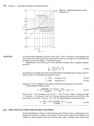
2.0 ^ g 6 Fig. 6.3-2. Graphical procedure used in
/ Example 6.3-1.
/
Line of slope 1.0 /
5
8 6 x l О" ! /
1.0 le /
0.8 /
0.6 /
Jo, —-?A - — —•
/
^ — — — - Porti on 0ffl /er 5Ш e
curv e frc>m Fig 6 3-Г
/ 0.4
/
0.3
/
0.2

0.1
10 4
2 ' 4
2.4 xlO 4
Re-

SOLUTION To find the sphere diameter, we have to solve Eq. 6.1-7 for D. However, in this equation one
has to know D in order to get /; and / is given by the solid curve in Fig. 6.3-1. A trial-and-error
procedure can be used, taking / = 0.44 as a first guess.
Alternatively, we can solve Eq. 6.1-7 for/and then note that //Re is a quantity indepen-
dent of D:

Psph - P
Re (6.3-18)
The quantity on the right side can be calculated with the information above, and we call it С
Hence we have two simultaneous equations to solve:
/=CRe from Eq. 6.3-18 (6.3-19)
/-/(Re) from Fig. 6.3-1 (6.3-20)
Equation 6.3-19 is a straight line with slope of unity on the log-log plot of/versus Re.
For the problem at hand we have

3
4 (980X9.58 X 1(T ) / .62 - 1.5<Л _ 5 .
2
C L 8 6 X 1 0 ( 6 3 2 1 )
~ 3 (i.59)(65)3 V 139 ; - "
5
Hence at Re = 10 , according to Eq. 6.3-19, / = 1.86. The line of slope 1 passing through
/ = 1.86 at Re = 10 is shown in Fig. 6.3-2. This line intersects the curve of Eq. 6.3-20 (i.e., the
5
4
curve of Fig. 6.3-1) at Re = Dv p//ji = 2.4 X 10 . The sphere diameter is then found to be
x
4
3
Re/x (2.4 x 10 )(9.58 x 10" )
D = = 2.2 cm (6.3-22)
pv, (1.59X65)
§6.4 FRICTION FACTORS FOR PACKED COLUMNS
In the preceding two sections we have discussed the friction factor correlations for two
simple flow systems of rather wide interest. Friction factor charts are available for a
number of other systems, such as transverse flow past a cylinder, flow across tube