Page 266 - Bird R.B. Transport phenomena

250 Chapter 8 Polymeric Liquids

between the stress tensor and the rate-of-strain tensor; for example, we can write the Jef-
freys model and then add some additional nonlinear terms for good measure:

т + A, j- т + W t r T)7 - h,{y • т + т • 7} = - Ц 7 + A y f у - ix \y • у}) (8.5-1)
2
t
2
in which the circumflexes О on the tensors indicate that their components are those
with respect to the corotating coordinate frame. In Eq. 8.5-1 the constants A lr A 2/ /% Mi/
and /JL all have dimensions of time.
2
Since the equations of continuity and motion are written for the usual xyz-coordinate
frame, fixed in space, it seems reasonable to transform Eq. 8.5-1 from the xyz frame into
the xyz frame. This is a purely mathematical problem, which was worked out long ago, 1
and the solution is well known. It can be shown that the partial time derivatives d/dt,
2
2
2
2
d /dt , • • • are changed into corotational (or Jaumann ' ) time derivatives %/Ш, ЯЬ /Ш ,
1 4
The corotational time derivative of a second-order tensor is defined as
in which со = Vv — (Vv) + is the vorticity tensor, and D/Dt is the substantial time deriva-
tive defined in §3.5. The tensor dot products appearing in Eq. 8.5-1, with components in
the xyz frame, transform into the corresponding dot products, with the components
given in the xyz frame.
When transformed into the xyz frame, Eq. 8.5-1 becomes

T + T + tr T T
^i G^7 2Mo( )7 ~ 2^il • 7 + 7 * т) = — T7 0 7 + A -=- у ~ /л [У ' 7J I (8.5-3)
2
2
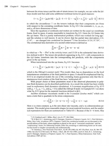
which is the Oldroyd 6-constant model. This model, then, has no dependence on the local
instantaneous orientation of the fluid particles in space. It should be emphasized that Eq.
8.5-3 is an empirical model; the use of the corotating frame guarantees only that the in-
stantaneous local rotation of the fluid has been "subtracted off."
With proper choice of these parameters most of the observed phenomena in poly-
mer fluid dynamics can be described qualitatively. As a result this model has been widely
used in exploratory fluid dynamics calculations. A 3-constant simplification of Eq. 8.5-3
with ^ = A lr /x 2 = A and /x 0 = 0 is called the Oldroyd-B model. In Example 8.5-1 we show
2/
what Eq. 8.5-3 gives for the material functions defined in §8.2.
5
Another nonlinear viscoelastic model is the 3-constant Giesekus model, which con-
tains a term that is quadratic in the stress components:
^ T - ^ T - 7 + 7 - T } J - a ^ | T - T = - ^ 7 (8.5-4)

Here A is a time constant, r] is the zero shear rate viscosity, and a is a dimensionless pa-
0
rameter. This model gives reasonable shapes for most material functions, and the analyt-
ical expressions for them are summarized in Table 8.5-1. Because of the {т • т} term, they

3
J. D. Goddard and С Miller, Rheol. Ada, 5,177-184 (1966).
4
R. B. Bird, R. C. Armstrong, and O. Hassager, Dynamics of Polymeric Liquids, Vol. 1, Fluid Mechanics,
Wiley, New York, 1st edition (1977), Chapters 7 and 8; the corotational models are not discussed in the
second edition of this book, where emphasis is placed on the use of "convected coordinates" and the
"codeforming" frame. For differential models, either the corotating or codeforming frame can be used,
but the former is simpler conceptually and mathematically.
5 H. Giesekus, /. Non-Newtonian Fluid Mech., 11, 69-109 (1982); 12, 367-374; Rheol. Ada, 21, 366-375
(1982). See also R. B. Bird and J. M. Wiest, /. Rheol, 29, 519-532 (1985), and R. B. Bird, R. C. Armstrong,
and O. Hassager, Dynamics of Polymeric Liquids, Vol. 1, Fluid Dynamics, Wiley-Interscience, New York,
2nd edition (1987), §7.3(c).