Page 268 - Bird R.B. Transport phenomena

252 Chapter 8 Polymeric Liquids

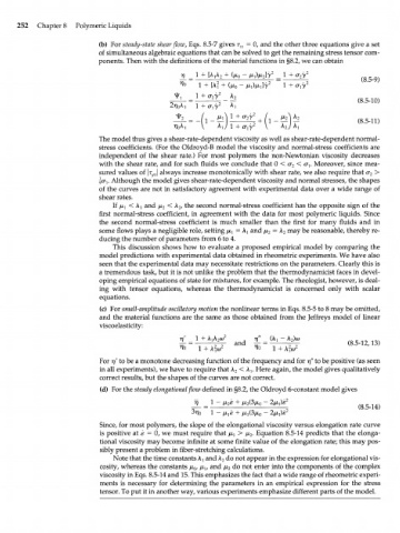
(b) For steady-state shear flow, Eqs. 8.5-7 gives r = 0, and the other three equations give a set
zz
of simultaneous algebraic equations that can be solved to get the remaining stress tensor com-
ponents. Then with the definitions of the material functions in §8.2, we can obtain
(Г2У 2
1 + [A? +

Lpy* _

A/ A (a5 n)
The model thus gives a shear-rate-dependent viscosity as well as shear-rate-dependent normal-
stress coefficients. (For the Oldroyd-B model the viscosity and normal-stress coefficients are
independent of the shear rate.) For most polymers the non-Newtonian viscosity decreases
with the shear rate, and for such fluids we conclude that 0 < cr < <Т\. Moreover, since mea-
2
sured values of \т \ always increase monotonically with shear rate, we also require that cr >
2
ух
\cr Although the model gives shear-rate-dependent viscosity and normal stresses, the shapes
v
of the curves are not in satisfactory agreement with experimental data over a wide range of
shear rates.
If /^ < AT and /JL 2 < A, the second normal-stress coefficient has the opposite sign of the
2
first normal-stress coefficient, in agreement with the data for most polymeric liquids. Since
the second normal-stress coefficient is much smaller than the first for many fluids and in
some flows plays a negligible role, setting ^ = \ and ц = А may be reasonable, thereby re-
l 2 2
ducing the number of parameters from 6 to 4.
This discussion shows how to evaluate a proposed empirical model by comparing the
model predictions with experimental data obtained in rheometric experiments. We have also
seen that the experimental data may necessitate restrictions on the parameters. Clearly this is
a tremendous task, but it is not unlike the problem that the thermodynamicist faces in devel-
oping empirical equations of state for mixtures, for example. The rheologist, however, is deal-
ing with tensor equations, whereas the thermodynamicist is concerned only with scalar
equations.
(c) For small-amplitude oscillatory motion the nonlinear terms in Eqs. 8.5-5 to 8 may be omitted,
and the material functions are the same as those obtained from the Jeffreys model of linear
viscoelasticity:

and ^-= V4 / 2 7 (8.5-12,13)
L 2
2
1 + A fa/ ^o 1 + Ao> 2
For 77' to be a monotone decreasing function of the frequency and for TJ" to be positive (as seen
in all experiments), we have to require that A < A^ Here again, the model gives qualitatively
2
correct results, but the shapes of the curves are not correct.
(d) For the steady elongational flow defined in §8.2, the Oldroyd 6-constant model gives

- ^ ^ (8.5-14)

Since, for most polymers, the slope of the elongational viscosity versus elongation rate curve
is positive at s = 0, we must require that ii x > fi . Equation 8.5-14 predicts that the elonga-
2
tional viscosity may become infinite at some finite value of the elongation rate; this may pos-
sibly present a problem in fiber-stretching calculations.
Note that the time constants X^ and A do not appear in the expression for elongational vis-
2
cosity, whereas the constants /x, \x and fx do not enter into the components of the complex
0
Xl
2
viscosity in Eqs. 8.5-14 and 15. This emphasizes the fact that a wide range of rheometric experi-
ments is necessary for determining the parameters in an empirical expression for the stress
tensor. To put it in another way, various experiments emphasize different parts of the model.