Page 304 - Bird R.B. Transport phenomena

288 Chapter 9 Thermal Conductivity and the Mechanisms of Energy Transport

9A.10. Thermal conductivity of chlorine-air mixtures.
6
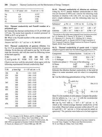
Metal k X 10 (ohm-cm) к (cal/cm • s • K)
e Using Eq. 9.3-17, predict thermal conductivities of chlo-
rine-air mixtures at 297 К and 1 atm for the following mole
Na 4.6 0.317
Ni 6.9 0.140 fractions of chlorine: 0.25, 0.50, 0.75. Air may be consid-
Cu 1.69 0.92 ered a single substance, and the following data may be
assumed:
Al 2.62 0.50
Substance" /.(Pa •s) fc(W/ i - K ) C (J/kg •K)
p
9A.8. Thermal conductivity and Prandtl number of a
polyatomic gas. Air 1.854 x 10" 5 2.614 X 1.001 X 10 3
(a) Estimate the thermal conductivity of CH at 1500K and Chlorine 1.351 X 10" 5 8.960 X 10" 3 4.798 X 10 2
4
1.37 atm. The molar heat capacity at constant pressure 4 at
a The entries in this table were prepared from functions provided
1500K is 20.71 cal/g-mole • K.
by T. E. Daubert, R. P. Danner, H. M. Sibul, С. С Stebbins,
(b) What is the Prandtl number at the same pressure and J. L. Oscarson, R. L. Rowley, W. V. Wilding, M. E. Adams,
temperature? T. L. Marshall, and N. A. Zundel, DIPPR ® Data Compilation of
4
Answers: (a) 5.03 X 10~ cal/cm • s • K; (b) 0.89 Pure Compound Properties, Design Institute for Physical Property
Data®, AlChE, New York (2000).
9A.9. Thermal conductivity of gaseous chlorine. Use
Eq. 9.3-15 to calculate the thermal conductivity of gaseous 9A.11. Thermal conductivity of quartz sand. A typical
chlorine. To do this you will need to use Eq. 1.4-14 to esti- sample of quartz sand has the following properties at 20°C:
mate the viscosity, and will also need the following values e
of the heat capacity: Component Volume fraction к cal/cm • s К
T(K) 200 300 400 500 600 i = l: Silica 0.510 20.4 X 10" 3
C p (cal/g-mole • K) (8.06) 8.12 8.44 8.62 6.74 i = 2: Feldspar 0.063 7.0 X 10" 3
Check to see how well the calculated values agree with the Continuous phase (i = 0) is one of the following:
following experimental thermal conductivity data 5 (i) Water 0.427 1.42 X 10" 3
(ii) Air 0.427 0.0615 X 10" 3
5
T(K) p (mm Hg) к X 10 cal/cm • s • К Estimate the effective thermal conductivity of the sand (i)
when it is water saturated, and (ii) when it is completely
198 50 1.31 ± 0.03 dry.
275 220 1.90 ± 0.02
276 120 1.93 ± 0.01 (a) Use the following generalization of Eqs. 9.6-5 and 6:
220 1.92 ± 0.01
363 100 2.62 ± 0.02 (9A.11-1)
200 2.61 ± 0.02 V N
395 210 3.04 ± 0.02 I
453 150 3.53 ± 0.03 /=0
250 3.42 ± 0.02 (9A.11-2)
495 250 3.72 ± 0.07
553 100 4.14 ± 0.04 Here N is the number of solid phases. Compare the predic-
583 170 4.43 ± 0.04 tion for spheres (g^ = g 2 = £з = I) with the recommenda-
210 4.45 ± 0.08 tion of de Vries (#, = g 2 = \; g 3 = f). 3
676 150 5.07 ± 0.10 (b) Use Eq. 9.6-1 with к л = 18.9 X 10~ cal/cm • s • K,
250 4.90 ± 0.03 which is the volume-average thermal conductivity of the
two solids. Observed values, accurate within about 3%, are
3
6.2 and 0.58 X 10~ cal/cm • s • К for wet and dry sand, re-
spectively. 6 The particles were believed to be best approxi-
4 O. A. Hougen, К. М. Watson, and R. A. Ragatz, Chemical
Process Principles, Vol. 1, Wiley, New York (1954), p. 253.
5 Interpolated from data of E. U. Frank, Z. Elektrochem., 55, 6 The behavior of partially wetted soil has been treated by
636 (1951), as reported in Nouveau Traitede Chimie Minerale, D. A. de Vries, Chapter 7 in Physics and Plant Environment,
ie
P. Pascal, ed., Masson et C , Paris (1960), pp. 158-159. W. R. van Wijk, ed., Wiley, New York (1963).