Page 332 - Bird R.B. Transport phenomena

316 Chapter 10 Shell Energy Balances and Temperature Distributions in Solids and Laminar Flow

Now let us evaluate the local heat transfer driving force, T o — T , which is the differ-
b
ence between the wall and bulk temperatures at a distance z down the tube:
rji rj-i 1 1 / U 1 1 (10.8-34)
io b
~ ~24X~48 к
where D is the tube diameter. We may now rearrange this result in the form of a dimen-
sionless wall heat flux
q D 48
0
k(T - T ) И (10.8-35)
0
b
which, in Chapter 14, will be identified as a Nusselt number.
Before leaving this section, we point out that the dimensionless axial coordinate £ in-
troduced above may be rewritten in the following way:

(10.8-36)
D{v z)p RePrlUJ Pe \R
Here D is the tube diameter, Re is the Reynolds number used in Part I, and Pr and Pe are
the Prandtl and Peclet numbers introduced in Chapter 9. We shall find in Chapter 11 that
the Reynolds and Prandtl numbers can be expected to appear in forced convection prob-
lems. This point will be reinforced in Chapter 14 in connection with correlations for heat
transfer coefficients.

§10.9 FREE CONVECTION
In §10.8 we gave an example of forced convection. In this section we turn our attention
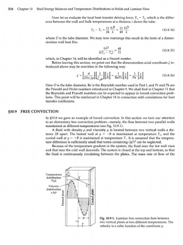
to an elementary free convection problem—namely, the flow between two parallel walls
maintained at different temperatures (see Fig. 10.9-1).
A fluid with density p and viscosity /л is located between two vertical walls a dis-
tance 2B apart. The heated wall at у = —В is maintained at temperature T , and the
2
cooled wall at у = +B is maintained at temperature T . It is assumed that the tempera-
}
1 2
ture difference is sufficiently small that terms containing (AT) can be neglected.
Because of the temperature gradient in the system, the fluid near the hot wall rises
and that near the cold wall descends. The system is closed at the top and bottom, so that
the fluid is continuously circulating between the plates. The mass rate of flow of the

Temperature
distribution

Velocity
distribution
v z {y)

Fig. 10.9-1. Laminar free convection flow between
two vertical plates at two different temperatures. The
velocity is a cubic function of the coordinate y.