Page 427 - Bird R.B. Transport phenomena

§13.2 The Time-Smoothed Temperature Profile Near a Wall 409

и)
in which it is understood that D/Dt = д/dt + v • V. Here q iv) = -kVT, and Ф[, is the vis-
cous dissipation function of Eq. B.7-1, but with all the v replaced by v r
{
In discussing turbulent heat flow problems, it has been customary to drop the vis-
cous dissipation terms. Then, one sets up a turbulent heat transfer problem as for lami-
(0
nar flow, except that т and q are replaced by т (у) + т (0 and q {v) + q , respectively, and
time-smoothed p, v, and T are used in the remaining terms.

§13.2 THE Т Ш Е - S M Q Q T H E D TEMPERATURE
PROFILE NEAR A WALL 1
Before giving empiricisms for q (0 in the next section, we present a short discussion of
some results that do not depend on any empiricism.
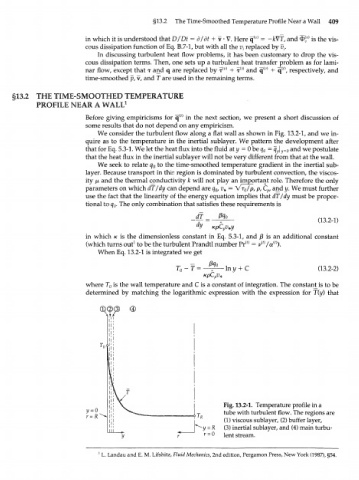
We consider the turbulent flow along a flat wall as shown in Fig. 13.2-1, and we in-
quire as to the temperature in the inertial sublayer. We pattern the development after
that for Eq. 5.3-1. We let the heat flux into the fluid at у = 0 be q = g | and we postulate
Q
y y=0
that the heat flux in the inertial sublayer will not be very different from that at the wall.
We seek to relate q to the time-smoothed temperature gradient in the inertial sub-
0
layer. Because transport in this region is dominated by turbulent convection, the viscos-
ity /x and the thermal conductivity к will not play an important role. Therefore the only
parameters on which dT/dy can depend are q , v* = Vr /p, p, C pf and y. We must further
o
0
use the fact that the linearity of the energy equation implies that dT/dy must be propor-
tional to q . The only combination that satisfies these requirements is
0
dT
(13.2-1)
in which к: is the dimensionless constant in Eq. 5.3-1, and /3 is an additional constant
(t)
1
{t)
(which turns out to be the turbulent Prandtl number Pr (0 = v /a ).
When Eq. 13.2-1 is integrated we get
-In у (13.2-2)

where T is the wall temperature and С is a constant of integration. The constants to be
o
determined by matching the logarithmic expression with the expression for T(y) that

Fig. 13.2-1. Temperature profile in a
tube with turbulent flow. The regions are
(1) viscous sublayer, (2) buffer layer,
(3) inertial sublayer, and (4) main turbu-
y
r = 0 lent stream.

1
L. Landau and E. M. Lifshitz, Fluid Mechanics, 2nd edition, Pergamon Press, New York (1987), §54.