Page 430 - Bird R.B. Transport phenomena

412 Chapter 13 Temperature Distributions in Turbulent Flow

I o o o o o o o o o o o o o o o o o o o o

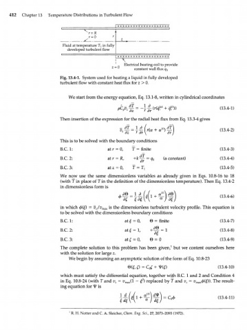
Fluid at temperature T in fully
7
developed turbulent flow
I o o o o o o o o o o o o o o o o o o o o
Electrical heating coil to provide
~ constant wall flux q 0
z
Fig. 13.4-1. System used for heating a liquid in fully developed
turbulent flow with constant heat flux for z > 0.

We start from the energy equation, Eq. 13.1-8, written in cylindrical coordinates

C v %= -jfr Щ^ + <7r°)) (13.4-1)
P p z
Then insertion of the expression for the radial heat flux from Eq. 13.3-4 gives

(13.4-2)
or/
This is to be solved with the boundary conditions
B.C.I: atr = 0, f = finite (13.4-3)
B.C. 2: atr = R, +k^- = q 0 (a constant) (13.4-4)
oT
B.C3: atz = 0, T = Т г (13.4-5)
We now use the same dimensionless variables as already given in Eqs. 10.8-16 to 18
(with T in place of Г in the definition of the dimensionless temperature). Then Eq. 13.4-2
in dimensionless form is
дв \ д ( ( ~ '
( л
±
in which ф(£) = v z/v max is the dimensionless turbulent velocity profile. This equation is
to be solved with the dimensionless boundary conditions

B.C. 1: at £ = 0, в = finite (13.4-7)
B.C. 2: at f = 1, + 4 ^ = 1 (13.4-8)
B.C3: at£ = 0, © = 0 (13.4-9)

The complete solution to this problem has been given, 1 but we content ourselves here
with the solution for large z.
We begin by assuming an asymptotic solution of the form of Eq. 10.8-23
в(€,0 = С<£ + П& (13.4-10)
which must satisfy the differential equation, together with B.C. 1 and 2 and Condition 4
2
in Eq. 10.8-24 (with T and v z = v (l - £ ) replaced by T and v z = У ф(О). The result-
max
тах
ing equation for 4? is

1
R. H. Notter and C. A. Sleicher, Chem. Eng. Sci., 27, 2073-2093 (1972).