Page 156 - Video Coding for Mobile Communications Efficiency, Complexity, and Resilience

Section 5.2. Warping-Based Methods: A Review 133

the reference frame are (u A ;v A ), (u B ;v B ), (u C ;v C ), and (u D ;v D ), respectively,
). Using the bilinear model of Equation
where, e.g., (u A ;v A )=(x A +d x A ;y A +d y A
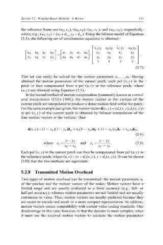
(5.5), the following set of simultaneous equations is obtained:


x A y A x B y B x C y C x D y D
u A u B u C u D a 1 a 2 a 3 a 4  x A x B x C x D 
= ·  :

v A v B v C v D a 5 a 6 a 7 a 8  y A y B y C y D 
1 1 1 1
(5.7)
This set can easily be solved for the motion parameters a 1 ;:::;a 8 . Having
obtained the motion parameters of the current patch, each pel (x; y)inthe
patch is then compensated from a pel (u; v) in the reference patch, where
(u; v) are obtained using Equation (5.5).
In the second method of motion compensation (commonly known as control
grid interpolation (CGI) [108]), the motion vectors at the vertices of the
current patch are interpolated to produce a dense motion (eld within the patch.
For the same example just given, the motion vector d(x; y)=(d x (x; y);d y (x; y))
at pel (x; y) of the current patch is obtained by bilinear interpolation of the
four motion vectors at the vertices. Thus

d(x; y)=(1 − x n )(1 − y n )d A + x n (1 − y n )d B +(1 − x n )y n d C + x n y n d D ;
(5.8)
x − x A y − y A
where x n = and y n = : (5.9)
x B − x A y C − y A
Each pel (x; y) in the current patch can then be compensated from pel (u; v)in
the reference patch, where (u; v)=(x + d x (x; y);y + d y (x; y)). It can be shown
[110] that the two methods are equivalent.

5.2.8 Transmitted Motion Overhead

Two types of motion overhead can be transmitted: the motion parameters a i
of the patches and the motion vectors of the nodes. Motion vectors have a
limited range and are usually evaluated to a (nite accuracy (e.g., full- or
half-pel accuracy), whereas motion parameters are not limited and are usually
continuous in value. Thus, motion vectors are usually preferred because they
are easier to encode and result in a more compact representation. In addition,
motion vectors ensure compatibility with current video coding standards. One
disadvantage in this case, however, is that the decoder is more complex, since
it must use the received motion vectors to calculate the motion parameters