Page 258 - Video Coding for Mobile Communications Efficiency, Complexity, and Resilience

Section 10.2. Temporal Error Concealment Using Motion Field Interpolation (MFI) 235

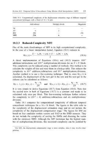
Table 10.1: Computational complexity of the displacement estimation stage of di,erent temporal
concealment techniques with a blockof 16 × 16 pels
Add=subtract Multiply=divide Magnitude

TR — — —
AV 6 2 —
BM 496 — 256
MFI 516 6 —

10.2.3 Reduced-Complexity MFI

One of the main disadvantages of MFI is its high computational complexity.
In the case of a linear interpolation kernel, Equation (10.1) reduces to

v ˆ(x; y)= (1 − x n )v L + x n v R +(1 − y n )v T + y n v B : (10.6)
2
A direct implementation of Equations (10.6) and (10.2) requires 10N 2
additions=subtractions and 12N multiplications=divisions for an N × N block.
2
This complexity can be reduced using a number of methods. One method is to
calculate the weights o,-line and store them in a lookup table. This reduces the
2
2
complexity to 6N additions=subtractions and 8N multiplications=divisions.
Another method is to use a line-scanning technique. That is, once v ˆ(x; y)is
calculated, the displacement of the next pel in the row and the next pel in the
column can be calculated as follows:
ˆ v(x +1;y)= ˆ v(x; y)+ v R − v L and ˆ v(x; y +1) = ˆ v(x; y)+ v B − v T : (10.7)
2N 2N
It is very simple to derive Equations (10.7) from Equation (10.6). Note that
the second term in both of Equations (10.7) is a constant and needs to be
calculated only once per block. This line-scanning technique further reduces
2
the complexity to (2N + 4) additions=subtractions and six multiplications=
divisions.
Table 10.1 compares the computational complexity of di,erent temporal
concealment techniques for a 16 × 16 block. The $gures in the table refer to
the complexity of the displacement estimation stage and do not include the
1
complexity of the displacement compensation stage. The $gures for BM are
based on four candidate motion vectors and SAD as the SMD measure. They
do not include the complexity of sorting the SMDs and choosing the vector
with the minimum SMD. Although the MFI technique has the highest num-
ber of multiplications=divisions, this increased complexity can be justi$ed by

1 For MFI, the displacement compensation stage is more complex, since it may involve inter-
polation.