Page 198 - Characterization and Properties of Petroleum Fractions - M.R. Riazi

QC: —/—
P2: KVU/KXT
P1: KVU/KXT
T1: IML
AT029-Manual-v7.cls
AT029-Manual
AT029-04
21:30
June 22, 2007
178 CHARACTERIZATION AND PROPERTIES OF PETROLEUM FRACTIONS
Solution—In Table 4.11 for C 12 and C 13 the mole fractions are
0.033 and 0.028, respectively. The molecular weights of these
components are 163 and 176. Therefore the average molec-
ular weight of the C 12 –C 13 group for this mixture is M av =
(0.033 × 163 + 0.028 × 176)/(0.033 + 0.028) = 169. The mole
fraction of these components is 0.033 + 0.028 or 0.061. Group
of C 12 –C 13 is referred to as subfraction i with average molec-
ular weight of M i,av and mole fraction of z i .
Equations (4.84) and (4.86) should be used to calculate z i
and M i,av , respectively. However, to use these equations, P i−1
and P i represent the lower and upper molecular weights of
the subfraction. In this case, the lower molecular weight is
M − and the upper limit is M . These values are given in
+
12 13
Table 4.10 as 156 and 184, respectively. P ∗ = (156 − 89.9)/
i−1
89.9 = 0.7353 and P = 1047. Substituting in Eq. (4.84) we
∗
i
get: z i = 0.059.
For this system, A = 0.3501 and B = 1; therefore, from
Eq. (4.87), q i−1 = 2.37048 and q i = 3.37401, which gives [39]
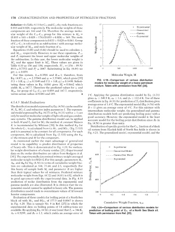
(1 + 1/B, q i−1 ) = 0.3149 and (1 + 1/B, q i ) = 0.1498. Substi- FIG. 4.19—Comparison of various distribution
tuting these values in Eq. (4.86) gives M = 0.8662 which models for molecular weight of a heavy petroleum
∗
n mixture. Taken with permission from Ref. [25].
yields M n = 167.7. Therefore the predicted values for z i and
M i,av for group of C 12 –C 13 are 0.059 and 167.7, respectively,
versus actual values of 0.061 and 169. 1 C. Applying the gamma distribution model by Eq. (4.31)
◦
gives η T = 349.9K, α T = 1.6, and β T = 112.4 K. Use of these
4.5.4.5 Model Evaluations coefficients in Eq. (4.31) for prediction of T b distribution gives
average error of 1.6 C. The exponential model (Eq. (4.56) with
◦
The distribution model expressed by Eq. (4.56) can be used for B = 1) gives an average error of 4 C. For this mixture with
◦
M, T b , SG, d, and refractive index parameter I. The exponen- intermediate molecular weight, the generalized and gamma
tial model expressed by Eq. (4.27) or Eq. (4.31) with α = 1 can distribution models both are predicting boiling point with a
only be used for molecular weight of light oils and gas conden- good accuracy. However, the exponential model is the least
sate systems. The gamma distribution model can be applied accurate model for the boiling point distribution since B T in
to both M and T b , but for SG, the method of constant Watson Eq. (4.56) is greater than unity.
K is recommended by Whitson [20]. In this method K W for Distribution of specific gravity for the C 7+ fraction of a black
the whole C 7+ is calculated from its M 7+ and SG 7+ (Eq. 2.133) oil system from Ekofisk field of North Sea fields is shown in
and it is assumed to be constant for all components. For each Fig. 4.21. The generalized model, exponential model, and the
component, SG is calculated from Eq. (2.133) using the K W
of the mixture and M for the component.
As mentioned earlier the main advantage of generalized
model is its capability to predict distribution of properties
of heavy oils. This is demonstrated in Fig. 4.19, for molecu-
lar weight distribution of a heavy residue [25]. Experimental
data on the molar distribution are taken from Rodgers et al.
[41]. The experimentally determined mixture weight averaged
molecular weight is 630 [41]. For this sample, parameters M o ,
A M , and B M for Eq. (4.56) in terms of cumulative weight frac-
tion are calculated as 144, 71.64, and 2.5, respectively. For
this heavy oil sample both M o and parameter B are higher
than their typical values for oil mixtures. Predicted mixture
molecular weight from Eqs. (4.72) and (4.81) is 632, which is
in good agreement with the experimental data. In Fig. 4.19
prediction of molar distribution from the exponential and
gamma models are also illustrated. It is obvious that the ex-
ponential model cannot be applied to heavy oils. The gamma
distribution model tends to overestimate values of M toward
heavier components.
Evaluation of these models for boiling point of a North Sea
black oil with M 7+ and SG 7+ of 177.5 and 0.8067 is shown
in Fig. 4.20. This is sample No. 8 in Ref. [25] in which the
experimental data on boiling points of 14 subfractions are FIG. 4.20—Comparison of various distribution models for
available. By applying Eq. (4.56), it was found that T o = 346 K, prediction of boiling point of C 7+ of a North Sea Black oil.
A T = 0.5299, and B T = 1.3, which yields an average error of Taken with permission from Ref. [25].

--`,```,`,``````,`,````,```,,-`-`,,`,,`,`,,`---
Copyright ASTM International
Provided by IHS Markit under license with ASTM Licensee=International Dealers Demo/2222333001, User=Anggiansah, Erick
No reproduction or networking permitted without license from IHS Not for Resale, 08/26/2021 21:56:35 MDT