Page 202 - Characterization and Properties of Petroleum Fractions - M.R. Riazi

P2: KVU/KXT
QC: —/—
T1: IML
P1: KVU/KXT
21:30
June 22, 2007
AT029-Manual-v7.cls
AT029-Manual
AT029-04
182 CHARACTERIZATION AND PROPERTIES OF PETROLEUM FRACTIONS
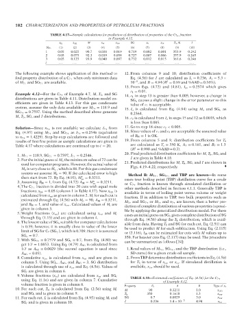
TABLE 4.17—Sample calculations for prediction of distribution of properties of the C 7+ fraction
in Example 4.12.
x m x cm M x w x cw SG x v x cv T b ,K I
No. (1) (2) (3) (4) (5) (6) (7) (8) (9) (10)
1 0.05 0.025 90.7 0.038 0.019 0.719 0.002 0.001 353.9 0.242
2 0.05 0.075 92.3 0.039 0.058 0.727 0.007 0.006 357.9 0.245
3 0.05 0.125 93.9 0.040 0.097 0.732 0.012 0.015 361.6 0.246
i ... ... ... ... ... ... ... ... ... ...
The following example shows application of this method to 12. From columns 9 and 10, distribution coefficients of
find property distribution of a C 7+ when only minimum data Eq. (4.56) for I are calculated as I o = 0.236, A I = 5.3 ×
2
−5
of M 7+ and SG 7+ are available. 10 , and B = 4.94 (R = 0.99 and %AAD = 0.16%).
13. From Eqs. (4.72) and (4.81), I av = 0.2574 which gives
ε 1 = 0.01.
Example 4.12—For the C 7+ of Example 4.7, M, T b , and SG 14. ε 1 in step 13 is greater than 0.005; however, a change in
distributions are given in Table 4.11. Distribution model co- SG o causes a slight change in the error parameter so this
efficients are given in Table 4.13. For this gas condensate value of ε 1 is acceptable.
system, assume the only data available are M 7+ = 118.9 and 15. I o is calculated from Eq. (4.94) using M o and SG o as
SG 7+ = 0.7597. Using the method described above generate 0.2364.
M, T b , SG, and I distributions. 16. ε 2 is calculated from I o in steps 15 and 12 as 0.0018, which
is less than 0.005.
Solution—Since n 7+ is not available we calculate I 7+ from 17. Go to step 18 since ε 2 < 0.005.
Eq. (4.95) using M 7+ and SG 7+ as I 7+ = 0.2546 (equivalent 18. Since values of ε 1 and ε 2 are acceptable the assumed value
to n 7+ = 1.4229). Step-by-step calculations are followed and of B M = 1isOK.
results of first few points as sample calculations are given in 19. From columns 5 and 9, distribution coefficients for T b
Table 4.17 where calculations are continued up to i = 20. are calculated as T o = 350 K, A T = 0.161, and B T = 1.3
2
(R = 0.998 and %AAD = 0.3).
20. Final predicted distribution coefficients for M, T b , SG, and
1. M 7+ = 118.9, SG 7+ = 0.7597, I 7+ = 0.2546.
2. For the initial guess of M o the minimum value of 72 can be I are given in Table 4.18.
used for computer programs. However, the actual value of 21. Predicted distributions for M, T b , SG, and I are shown in
M o is very close to M , which is 88. For this gas condensate Figs. 4.19–4.22, respectively.
−
7
system we assume M o = 90. If the calculated error is high Method B: M 7++ , SG 7++ , and TBP are known—In some
then start from 72. By Eq. (4.93), M = 0.3211. cases true boiling point (TBP) distillation curve for a crude
∗
av
3. Assuming B M = 1, from Eq. (4.72) A M = M = 0.3211. or C 7+ fraction is known through simulated distillation or
∗
av
4. The C 7+ fraction is divided into 20 cuts with equal mole other methods described in Section 4.1.1. Generally TBP is
fractions: x mi = 0.05 (column 1 in Table 4.17). Now x cm is available in terms of boiling point versus volume or weight
calculated from x wi as given in column 2. M i for each cut is fraction. If in addition to TBP, two bulk properties such as
estimated through Eq. (4.56) with M o = 90, A M = 0.3211, M 7+ and SG 7+ or M 7+ and n 7+ are known, then a better pre-
and B M = 1, and value of x cm . Calculated values of M i are diction of complete distribution of various properties is possi-
given in column 3.
ble by applying the generalized distribution model. For these
5. Weight fractions (x wi ) are calculated using x mi and M i cases an initial guess on SG o gives complete distribution of SG
through Eq. (1.15) and are given in column 4. through Eq. (4.56) along the T b distribution, which is avail-
--`,```,`,``````,`,````,```,,-`-`,,`,,`,`,,`---
6. The lowest value of SG o suitable for computer calculations able from data. Having T b and SG for each cut, Eq. (2.51) can
is 0.59; however, it is usually close to value of the lower be used to predict M for each subfraction. Using Eq. (2.115)
−
limit of SG for C 7 (SG ), which is 0.709. Here it is assumed
7 or (2.116), I 20 can be estimated for cuts with M values up to
SG o = 0.7. 350. For heavier cuts Eq. (2.117) may be used. The procedure
7. With SG 7+ = 0.7579 and SG o = 0.7, from Eq. (4.80) we can be summarized as follows [24]:
get 1/J = 1.0853. Using Eq. (4.79) A SG is calculated from
1/J as A SG = 0.0029 (the second equation is used since 1. Read values of M 7+ ,SG 7+ , and the TBP distribution (i.e.,
A SG < 0.05). SD curve) for a given crude oil sample.
8. Cumulative x cw is calculated from x wi and are given in 2. From TBP determine distribution coefficients in Eq. (4.56)
column 5. Using SG o , A SG , and B SG = 3, SG distribution for T b in terms of x cw or x cv . If simulated distillation is
is calculated through use of x cw and Eq. (4.56). Values of available, x cw should be used.
SG i are given in column 6.
9. Volume fractions (x vi ) are calculated from x wi and SG i
using Eq. (1.16) and are given in column 7. Cumulative TABLE 4.18—Estimated coefficients of Eq. (4.56) for the C 7+
of Example 4.12.
volume fraction is given in column 8. Property P o A B Type of x c
10. For each cut, T bi is calculated from Eq. (2.56) using M i M 90 0.3211 1.0 x cm
and SG i and is given in column 9. T b 350 0.1610 1.3 x cw
11. For each cut, I i is calculated from Eq. (4.95) using M i and SG 0.7 0.0029 3.0 x cw
SG i and is given in column 10. I 0.236 5.4 × 10 −5 4.94 x cv

Copyright ASTM International
Provided by IHS Markit under license with ASTM Licensee=International Dealers Demo/2222333001, User=Anggiansah, Erick
No reproduction or networking permitted without license from IHS Not for Resale, 08/26/2021 21:56:35 MDT