Page 205 - Characterization and Properties of Petroleum Fractions - M.R. Riazi

QC: —/—
T1: IML
P1: KVU/KXT
P2: KVU/KXT
AT029-Manual-v7.cls
June 22, 2007
21:30
AT029-04
AT029-Manual
4. CHARACTERIZATION OF RESERVOIR FLUIDS AND CRUDE OILS 185
application of Gaussian quadrature technique as discussed
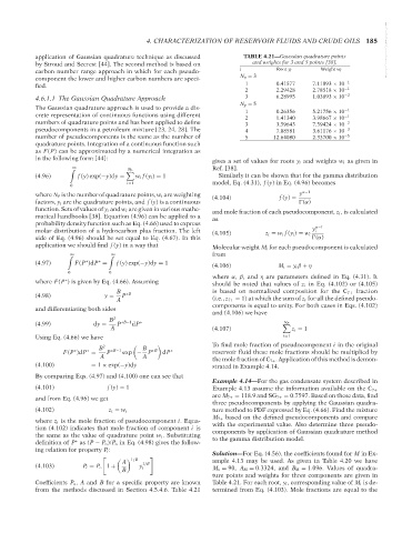
and weights for 3 and 5 points [38].
by Stroud and Secrest [44]. The second method is based on TABLE 4.21—Gaussian quadrature points --`,```,`,``````,`,````,```,,-`-`,,`,,`,`,,`---
carbon number range approach in which for each pseudo- i Root y i Weight w i
component the lower and higher carbon numbers are speci- N p = 3 −1
fied. 1 0.41577 7.11093 × 10
2 2.29428 2.78518 × 10 −1
4.6.1.1 The Gaussian Quadrature Approach 3 6.28995 1.03893 × 10 −2
N p = 5
The Gaussian quadrature approach is used to provide a dis- 1 0.26356 5.21756 × 10 −1
crete representation of continuous functions using different 2 1.41340 3.98667 × 10 −1
numbers of quadrature points and has been applied to define 3 3.59643 7.59424 × 10 −2
pseudocomponents in a petroleum mixture [23, 24, 28]. The 4 7.08581 3.61176 × 10 −3
number of pseudocomponents is the same as the number of 5 12.64080 2.33700 × 10 −5
quadrature points. Integration of a continuous function such
as F(P) can be approximated by a numerical integration as
in the following form [44]:
gives a set of values for roots y i and weights w i as given in
∞ Ref. [38].
N p

(4.96) f (y) exp(−y)dy = w i f (y i ) = 1 Similarly it can be shown that for the gamma distribution
i=1 model, Eq. (4.31), f (y) in Eq. (4.96) becomes
0
where N P is the number of quadrature points, w i are weighting (4.104) y α−1
factors, y i are the quadrature points, and f (y) is a continuous f (y) = (α)
function. Sets of values of y i and w i are given in various mathe- and mole fraction of each pseudocomponent, z i , is calculated
matical handbooks [38]. Equation (4.96) can be applied to a as
probability density function such as Eq. (4.66) used to express α−1
molar distribution of a hydrocarbon plus fraction. The left (4.105) z i = w i f (y i ) = w i y i
side of Eq. (4.96) should be set equal to Eq. (4.67). In this (α)
application we should find f (y) in a way that Molecular weight M i for each pseudocomponent is calculated
from
∞ ∞

(4.97) F(P )dP = f (y) exp(−y)dy = 1 (4.106) M i = y i β + η
∗
∗
0 0
where α, β, and η are parameters defined in Eq. (4.31). It
where F(P ) is given by Eq. (4.66). Assuming should be noted that values of z i in Eq. (4.102) or (4.105)
∗
B is based on normalized composition for the C 7+ fraction
(4.98) y = P ∗B
A (i.e., z 7+ = 1) at which the sum of z i for all the defined pseudo-
components is equal to unity. For both cases in Eqs. (4.102)
and differentiating both sides
and (4.106) we have
B 2
(4.99) dy = P ∗B−1 dP ∗
N P
A (4.107) z i = 1
Using Eq. (4.66) we have i=1
To find mole fraction of pseudocomponent i in the original
2
B B

∗ ∗ ∗B−1 ∗B ∗
F(P )dP = P exp − P dP reservoir fluid these mole fractions should be multiplied by
A A
the mole fraction of C 7+ . Application of this method is demon-
(4.100) = 1 × exp(−y)dy strated in Example 4.14.
By comparing Eqs. (4.97) and (4.100) one can see that
Example 4.14—For the gas condensate system described in
(4.101) f (y) = 1
Example 4.13 assume the information available on the C 7+
and from Eq. (4.96) we get are M 7+ = 118.9 and SG 7+ = 0.7597. Based on these data, find
three pseudocomponents by applying the Gaussian quadra-
(4.102) z i = w i ture method to PDF expressed by Eq. (4.66). Find the mixture
M 7+ based on the defined pseudocomponents and compare
where z i is the mole fraction of pseudocomponent i. Equa-
tion (4.102) indicates that mole fraction of component i is with the experimental value. Also determine three pseudo-
the same as the value of quadrature point w i . Substituting components by application of Gaussian quadrature method
definition of P as (P − P o )/P o in Eq. (4.98) gives the follow- to the gamma distribution model.
∗
ing relation for property P i :
Solution—For Eq. (4.56), the coefficients found for M in Ex-

A 1/B
1/B ample 4.13 may be used. As given in Table 4.20 we have
(4.103) P i = P ◦ 1 + y i M o = 90, A M = 0.3324, and B M = 1.096. Values of quadra-
B
ture points and weights for three components are given in
Coefficients P o , A and B for a specific property are known Table 4.21. For each root, y i , corresponding value of M i is de-
from the methods discussed in Section 4.5.4.6. Table 4.21 termined from Eq. (4.103). Mole fractions are equal to the
Copyright ASTM International
Provided by IHS Markit under license with ASTM Licensee=International Dealers Demo/2222333001, User=Anggiansah, Erick
No reproduction or networking permitted without license from IHS Not for Resale, 08/26/2021 21:56:35 MDT