Page 257 - Mechanical Behavior of Materials

258 Chapter 6 Review of Complex and Principal States of Stress and Strain

Example 6.6
For the same state of stress as in Ex. 6.3, determine the principal normal stresses by treating
this as a three-dimensional problem. Recall that the given state of stress is σ x = 100,σ y =
−60,σ z = 40,τ xy = 80, and τ yz = τ zx = 0MPa.
Solution Substitute these given stresses into Eq. 6.29 to obtain values for the stress invariants:

I 1 = 80, I 2 =−10,800, I 3 =−496,000

These values correspond to units of MPa for stresses, as employed throughout this solution. The
cubic relationship of Eq. 6.28 is thus

3 2 3 2
σ − σ I 1 + σ I 2 − I 3 = 0, σ − 80σ − 10,800σ + 496,000 = 0

For a number of values of σ, calculate the corresponding values of f (σ):

2
3
σ − 80σ − 10,800σ + 496,000 = f (σ)
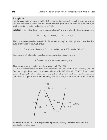
Then use these values to plot the cubic equation as in Fig. E6.6.
It is evident that there are three roots where the curve crosses the σ-axis, where f (σ) = 0.
From the graph, these roots can be seen to be roughly 130, 40, and −90 MPa. Starting with
each of these rough values in turn, apply trial and error, Newton’s method, or another numerical
procedure, as implemented in various widely available computer software. Accurate values are

f (σ)
5
8 x 10

4

40
–100 100 200
σ, MPa
0
–93.1 σ = 133.1
–4

Figure E6.6 Graph of the example cubic equation, showing the three roots that are
principal normal stresses.