Page 112 - Introduction to Statistical Pattern Recognition

94 Introduction to Statistical Pattern Recognition

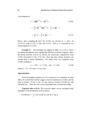
c are computed as

(3.137)

That is, after computing p and L by (3.129), we calculate hi, vi, and c of
(3.127) by using (3.135), (3.136), and (3.137). Then is computed by the
second equation of (3.128).

Example 11: The technique was applied to Data I-A (n =8) in which
two normal distributions have significantly different covariance matrices. First,
the density functions of h for ol and o2 are numerically computed by using
(3.110) and plotted in Fig. 3-16 [14]. Note that these density functions are
skewed from a normal distribution. The Bayes error was computed using
(3.128), resulting in
= 1.6%, = 2.2%, and E = 1.9% , (3.138)

where P I = P2 = 0.5 and t = 0 are used.

Approximations

Since the quadratic equation of (3.1 1) represents the summation of many
terms, the central limit theorem suggests that the distribution of h (X) could be
close to normal. If that is true, we only need to compute E(h(X)loj) and
Var{ h (X) I wi ). Then, the error can be calculated from a normal error table.

Expected value of h(X): The expected values can be calculated easily
regardless of the distributions of X as follows:
1
E(h(X)Iwl) = - tr [~.;'E((x-M~)(x-M,)'I~~ 11
2